Impacts of Hyperbolic Discounting on Inventory Replenishment Policy Under Inflation

1 Introduction

The increasing consumer price index indicates the strengthening severity of inflation these years in China. We realize that on the one hand, inventory replenishment policy is greatly influenced by the external macroeconomics; on the other hand, it’s also explicitly impacted by the decision maker’s subjective perception, such as his or her degree of confidence towards future value of money and anxiety to return the money. Over the planning time horizon, given the objective indicator, say, the compounded discount rate, the decision maker may prefer the conservative replenishment policy, when his or her confidence perceived towards future value of money is decreasing and anxiety to return the money is increasing. Moreover, when inflation is more severe, the decision maker may not be patient and rational any more. Instead, he or she may become anxious and eager to return the money and gain the immediate benefit by adjusting inventory replenishment policy. That’s to say, the decision maker will focus on the present, instead of the future, to acquire immediate reward. How can we reflect these characteristics in the inventory replenishment model? How do the degree of confidence and anxiety change inventory replenishment policy? How can we combine the subjective perception of the decision maker with the objective indicator from the capital market, to make better inventory decisions? The traditional inventory replenishment models don’t provide with us the lens through which we can look into these issues effectively.

Trading off cost and benefit over time, people actually have bounded rationality and reveal time inconsistency. That’s, people’s preference for future reward may change over time and the temptation of immediate reward can be considerably irresistible[1–5]. Plenty of psychological experiments and economic literature have supported these characteristics[6–12]. When making inter-temporal decisions, people outweigh the present, compared with the future. When setting inter-temporal preference, their valuation of the outcome will be more discounted over time[13–16]. The decision maker, who is making inventory replenishment policy under inflation, also shows time inconsistency and inter-temporal preference when making inter-temporal choices. The effect of time inconsistency and inter-temporal preference will be more salient when inflation is more severe. Time inconsistency and inter-temporal preference can be represented by hyperbolic discounting[17].

For hyperbolic discounting function, its discount rate is γ/(1 + αt), and a reward at future time t will be discounted by the factor (1 + αt)^−γ/α, where α and γ are positive[18−19]. Compared with the constant discount rate under exponential discounting, the discount rate of hyperbolic discounting is declining with regard to time t. This feature implies time inconsistency of the decision maker when making inter-temporal decisions. Due to analytical intractability of hyperbolic discounting function, quasi-hyperbolic discounting function is popularly employed[20]. For the discrete quasi-hyperbolic discounting function, the discount factor is given as

where time interval [0,τ₀) is the present with exponential discounting and time internal [τ₀, ∞) is the future with exponential discounting multiplying an factor α (0 ≤ α ≤ 1). Besides, the length of the present τ₀ is stochastic and exponentially distributed with hazard rate λ (λ ≥ 0). For the continuous quasi-hyperbolic discounting function, the discount factor is given as

implying that D(t) is a linear combination of the exponential discount factor e^−γt with weight α and the exponential discount factor e^{−(γ + λ)t} with weight (1 − α). In our inventory models to reveal the decision maker’s time inconsistency, we use continuous quasi-hyperbolic discounting function only.

Hyperbolic discounting has received some applications and provided valuable insights in behavioral operations management[21−23]. Recently, for revenue-management problem, Su[24] considered customers’ emphases on the immediate cost relative to the future benefit. For service systems, Huang et al.[25] studied customers’ bounded rationality. Plambeck and Wang[26] presented the optimal pricing and scheduling for an unpleasant service generating long-term future benefits. For the newsvendor model, Chen et al.[27] analyzed the role of mental accounting on the effect of payment schemes on inventory decisions. In this paper, we research the impacts of hyperbolic discounting on inventory replenishment policy.

Literature on the economic order quantity (EOQ) models with different demand function under inflation is abounding[28−31]. All of these models are under exponential discounting, which assumes absolute rationality and neglects time inconsistency of the decision maker. For the non-deteriorating item, Trippi and Lewin[32] initially exercised the discounted cash flow (DCF) approach to get present value of the average inventory cost over the infinite time horizon. Moon and Yun[33] introduced the DCF approach to consider the situation where the finite planning horizon is a random variable. Hariga[34] considered the replenishment policy with time continuous non-stationary demand over a given finite planning horizon. For the deteriorating item[35−36], Bose[37] took account of the EOQ model where demand is linear time-dependent and shortages are allowed. Chung and Liu[38] explored a line search technique to decide the optimal interval over the finite time horizon. Chung and Lin[39] investigated optimal inventory replenishment policy without shortage and with shortages completely backlogged where demand is stable. Moon et al.[40] took ameliorating/deteriorating items into account where demand is time-varying. Gilding[41] formulated optimal inventory replenishment schedule subject to time-dependent demand and inflation, with no restriction on the timing of the orders or the start of the shortage periods . In this paper, however, we employ hyperbolic discounting to consider time value of money for the deteriorating item over the given planning time horizon. We research the impacts of time inconsistency and inter-temporal preference of the decision maker on inventory replenishment policy. Besides, we consider the cases with stable demand where there is no shortage and there are shortages with complete backlogging.

The rest of this paper is organized as follows. Section 2 presents the description of the models. Section 3 formulates mathematical models in the case of no shortage and shortages with complete backlogging, respectively. Section 4 provides numerical examples. Section 5 comes to the conclusions and managerial insights.

2 Model Description

Over a given finite planning time horizon under inflation, the decision maker is facing the problem of how to determine the optimal order frequency and order quantity in each ordering cycle, so as to maximize present value of total profit. All the costs and sales revenue are discounted by continuous quasi-hyperbolic discounting . Total cost includes fixed ordering cost, procurement cost, inventory holding cost and shortages cost (if shortages are allowed); total revenue is from selling items; total profit is the difference between total revenue and total cost.

Assumptions:

1. Time horizon is finite and lead time is zero;

2. Demand rate of single items is constant and replenishment rate of items is infinite;

Notation:

H Finite planning time horizon;

T Length of ordering cycle, decision variable;

n Order frequency, decision variable, n = H/T;

Q Order quantity, decision variable;

T_j Total elapsed time including the jth ordering cycle (j = 1, 2, ⋯, n), denoting the occurrence of the (j + 1)th ordering. T_j = jH/n = jT, where T_j = H and T₀ = 0;

t_j The time at which the inventory level in the jth ordering cycle drops to zero in the case of shortages (j = 1, 2, ⋯, n);

A Fixed ordering cost per ordering;

d Demand rate;

p Sale price per unit;

c Procurement cost per unit;

h Inventory holding cost per unit per time;

s Shortage cost per unit per time;

θ Deterioration rate, 0 < θ ≤ 1;

γ Compounded discount rate, net of inflation, 0 ≤ γ ≤ 1;

λ Hazard rate, λ ≥ 0;

α Confidence of the decision maker towards future value of money, 0 ≤ α ≤ 1.

3 Mathematical Models

Discount factor at any time t with continuous quasi-hyperbolic discounting is given as

Let β = 1 − α, η = γ + λ, then D(t) = α e^−γt + β e^−ηt. Thus, quasi-hyperbolic discounting could be regarded as the linear combination of exponential discounting e^−γt with the discounted weight α and exponential discounting e^−ηt with the discounted weight β. Here, make it clear that α denotes confidence of the decision maker towards future value of money. A smaller α means that the decision maker show less confidence towards future value of money, and the same amount of money in the future will be more depreciated than that under constant discount rate. λ presents hazard rate, which could be understood as how soon the future perceived by the decision maker will come. A larger λ means that the sooner the future will come and the more anxiety the decision maker will have. We use parameter α and λ to reflect the decision maker’s time inconsistency when facing inter-temporal choices.

3.1 No Shortage

In this subsection, we assume that shortages are not allowed.

Figure 1 shows the pattern of inventory level without shortage over the given planning time horizon H.

Figure 1

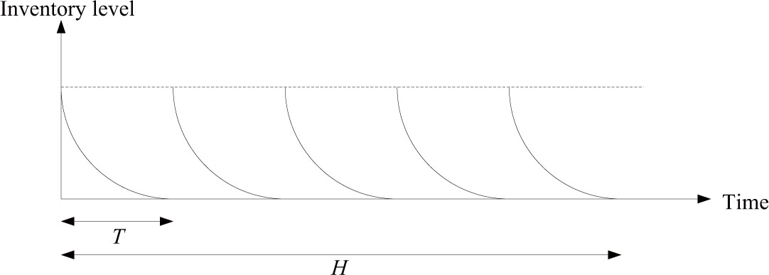
Inventory level of deteriorating items without shortage

The instantaneous inventory level I(t) during the first ordering cycle is regulated by

dI(t)dt=−θI(t)−d,0≤t≤T.(1)

For I(T) = 0, solution to (1) will be

I(t)=d[eθ(T−t)−1]θ,0≤t≤T.(2)

Present value of holding cost during the first ordering cycle is

CH1=h∫0TI(t)D(t)dt=αh∫0Td[eθ(T−t)−1]θe−γtdt+βh∫0Td[eθ(T−t)−1]θe−ηtdt=αhdθ(eθH/n−e−γH/nθ+γ+e−γH/n−1γ)+βhdθ(eθH/n−e−ηH/nθ+η+e−ηH/n−1η),(3)

and present value of holding cost over the entire time horizon H is

CH=αhdθ(eθH/n−e−γH/nθ+γ+e−γH/n−1γ)∑j=1ne−γTj−1+βhdθ(eθH/n−e−ηH/nθ+η+e−ηH/n−1η)∑j=1ne−ηTj−1=αhdθ(eθH/n−e−γH/nθ+γ+e−γH/n−1γ)1−e−γH1−e−γH/n+βhdθ(eθH/n−e−ηH/nθ+η+e−ηH/n−1η)1−e−ηH1−e−ηH/n.(4)

Present value of ordering cost over the entire time horizon H is

CO=A(∑j=1nαe−γTj−1+∑j=1nβe−ηTj−1)=αA1−e−γH1−e−γH/n+βA1−e−ηH1−e−ηH/n.(5)

Present value of procurement cost over the entire time horizon H is

CP=cI(0)(∑j=1nαe−γTj−1+∑j=1nβe−ηTj−1)=cdθ(eθH/n−1)(∑j=1nαe−γTj−1+∑j=1nβe−ηTj−1)=αcdθ(eθH/n−1)1−e−γH1−e−γH/n+βcdθ(eθH/n−1)1−e−ηH1−e−ηH/n.(6)

Hence, present value of total cost over the entire time horizon H is

TC=CH+CO+CP.(7)

Present value of revenue during the first ordering cycle is

R=p∫0TdD(t)dt=pd∫0T(αe−γt+βe−ηt)dt=αpdγ(1−e−γH/n)+βpdη(1−e−η),(8)

and present value of total revenue over the entire time horizon H is

TR=αpdγ(1−e−γH/n)∑j=1ne−γTj−1+βpdη(1−e−ηH/n∑j=1ne−ηTj−1=αpdγ(1−e−γH/n)1−e−γH1−e−γH/n+βpdη(1−e−ηH/n)1−e−ηH1−e−ηH/n.(9)

Hence, present value of total profit over the entire time horizon H is

TP=TR−TC.(10)

Combining all the above equations and rearrange the results, we obtain

TP(n)=α{pdγ(1−e−γH/n)−cdθ(eθH/n−1)−hdθ(eθH/n−e−γH/nθ+γ+e−γH/n−1γ)−A}1−e−γH1−e−γH/n+β{pdη1−e−ηH/n)−cdθ(eθH/n−1)−hdθ(eθH/n−e−ηH/nθ+η+e−ηH/n−1η)−A}1−e−ηH1−e−ηH/n.(11)

Theorem 1

Present value of total profit function TP(n) is concave with regard to n.

Before proving Theorem 1, let

TC(n)={cdθ(eθH/n−1)+hdθ(eθH/n−e−γH/nθ+γ+e−γH/n−1γ)+A}1−e−γH1−e−γH/n,

then we have the following lemma.

Lemma 1

Function TC(n) is convex with regard to n.

Proof

Following a similar way used by Chung and Lin[39], one can easily derive Lemma 1. We omit the proof for brevity.

In what follows, we show the proof of Theorem 1. According to Lemma 1, −TC(n) is concave with regard to n.

Let

TP1(n)={pdγ(1−e−γH/n−cdθ(eθH/n−1)−hdθ(eθH/n−e−γH/nθ+γ+e−γH/n−1γ)−A}1−e−γH1−e−γH/n,TP1(n)={pdη(1−e−ηH/n−cdθ(eθH/n−1)−hdθ(eθH/n−e−ηH/nθ+η+e−ηH/n−1η)−A}1−e−ηH1−e−ηH/n,

then TP₁ (n) and TP₂ (n) is concave with regard to n, respectively.

Therefore, TP(n), the linear combination of TP₁(n) and TP₂ (n), is concave with regard to n. We complete the proof of Theorem 1.

Based on Theorem 1, the solution procedure to determine the optimal order frequency n^* and present value of total profit TP(n^*) is provided by the following algorithm.

Algorithm 1

Step 1 Input the values of all the parameters, and set TP(0) = 0 and n = 1;

Step 2 Calculate TP(n) from (11);

Step 3 If TP(n) > TP(n − 1), then set n = n + 1 and go back to Step 2; otherwise, stop and set n^* = n − 1.

Thus, we get the optimal order frequency n^*, and the optimal present value of total profit TP(n^*). The optimal order quantity in each ordering cycle and length of ordering cycle are given as Q^* = dθ (e^θH/n* − 1), T^* = H/n^*.

3.2 Shortages with Complete Backlogging

In this subsection, we assume that shortages are allowed and completely backlogged.

With shortages allowed, suppose that (n + 1) orderings are conducted over the given time horizon H. The last replenishment is made at time t = H, only to replenish the last shortage quantity produced in the last cycle. Assume that in each ordering cycle [T_j−1, T_j] (j = 1, 2, ⋯, n−1), there are no-shortage period KT (0 < K < 1) and shortage period (1 − K)T. Shortages occur at time t_j = (K + j − 1)T (j = 1, 2, ⋯, n − 1).

Figure 2 shows the pattern of inventory level with shortages completely backlogged over the given planning time horizon H.

Figure 2

Inventory level of deteriorating items with shortages

The instantaneous inventory level I(t) of the no-shortage period is ruled by

dI(t)dt=−θI(t)−d,0≤t≤t1.(12)

The shortages inventory level S(t) is governed by

dS(t)dt=−d,t1≤t≤T.(13)

For I(T) = 0, solutions to (12) and (13) will be

I(t)=d[eθ(t1−t)−1]θ,0≤t≤t1,(14)

S(t)=d(t−t1),t1≤t≤T.(15)

Let I₀ and S₀ be the initial inventory level and the maximum shortage quantity, respectively, then we have

I0=dθ(eθKH/n−1),(16)

S0=dH(1−K)n.(17)

Present value of holding cost during the first ordering cycle is

CH1=h∫0t1I(t)D(t)dt=αh∫0t1d[eθ(t1−t)−1]θe−γtdt+β∫0t1d[eθ(t1−t)−1]θe−ηtdt=αhdθ(eθKH/n−e−γKH/nθ+γ+e−γKH/n−1γ)+βhdθ(eθKH/n−e−ηKH/nθ+η+e−ηKH/n−1η),(18)

and present value of holding cost over the entire time horizon H is

CH=αhdθ(eθKH/n−e−γKH/nθ+γ+e−γKH/n−1γ)∑j=1ne−γTj−1+βhdθ(eθKH/n−e−ηKH/nθ+η+e−ηKH/n−1η)∑j=1ne−ηTj−1=αhdθ(eθKH/n−e−γKH/nθ+γ+e−γKH/n−1γ)1−e−γH1−e−γH/n+βhdθ(eθKH/n−e−ηKH/nθ+η+e−ηKH/n−1η)1−e−ηH1−e−ηH/n.(19)

Present value of shortage cost during the first ordering cycle is

CS1=s∫t1TS(t)D(t)dt=αs∫t1Td(t−t1)e−γtdt+βs∫t1Td(t−t1)e−ηtdt=αsdγ2[γH(K−1)n+eγ(1−K)H/n−1]+βsdη2[ηH(K−1)n+eη(1−K)H/n−1],(20)

and present value of shortage cost over the entire time horizon H is

CS=αsdγ2[γH(K−1)n+eγH(1−K)/n−1]∑j=1ne−γTj−1+βsdη2[ηH(K−1)n+eηH(1−K)/n−1]∑j=1ne−ηTj−1=αsdγ2[γH(K−1)n+eγH(1−K)/n−1]1−e−γH1−e−γH/n+βsdη2[ηH(K−1)n+eηH(1−K)/n−1]1−e−ηH1−e−ηH/n.(21)

Present value of ordering cost over the entire time horizon H is

CO=A∑j=0n(αe−γTj+βe−ηTj)=αAeγH/n−e−γHeγH/n−1+βAeηH/n−e−ηHeηH/n−1.(22)

Present value of procurement cost over the entire time horizon H is

CP=cI0∑j=1n(αe−γTj−1+βe−ηTj−1)+cS0∑j=1n(αe−γTj+βe−ηTj)=cdθ(eθH/n−1)∑j=1n(αe−γTj−1+βe−ηTj−1)+cdH(1−K)n∑j=1n(αe−γTj+βe−ηTj)=αcdθ(eθKH/n−1)1−e−γH1−e−γH/n+βcdθ(eθKH/n−1)1−e−ηH1−e−ηH/n+αcdH(1−K)n1−e−γHeγH/n−1+βcdH(1−K)n1−e−ηHeηH/n−1.(23)

Hence, present value of total cost over the entire time horizon H is given as

TC=CH+CO+CP+CS.(24)

Present value of revenue during the first ordering cycle is

R=pd∫0t1D(t)dt=αpd∫0t1e−γtdt+βpd∫0t1e−ηtdt=αpdγ(1−e−γKH/n)+βpdη(1−e−ηKH/n),(25)

and present value total revenue over the entire time horizon H is given as

TR=αpdγ(1−e−γKH/n)∑j=1ne−γTj−1+βpdη1−e−ηKH/n)∑j=1ne−ηTj−1+pdH(1−K)n(∑j=1nαe−γTj+∑j=1nβe−ηTj)=αpdγ(1−e−γKH/n)1−e−γH1−e−γH/n+βpdη(1−e−ηKH/n)1−e−ηH1−e−ηH/n+αpdH(1−K)n1−e−γHeγH/n−1+βpdH(1−K)n1−e−ηHeηH/n−1.(26)

Hence, present value of total profit over the entire time horizon H is

TP=TR−TC.(27)

Combining all the above equations and rearrange the results, we obtain

TP(n,K)=αd{pγ(1−e−γKH/n)−cθ(eθKH/n−1)−hθ(eθKH/n−e−γKH/nθ+γ+e−γKH/n−1γ)−sγ2[γH(K−1)n+eγH(1−K)/n−1]}1−e−γH1−e−γH/n+βd{pη(1−e−ηKH/n)−cθ(eθKH/n−1)−hθ(eθKH/n−e−ηKH/nθ+η+e−ηKH/n−1η)−sη2[ηH(K−1)n+eηH(1−K)/n−1]}1−e−ηH1−e−ηH/n+α(p−c)dH(1−K)n1−e−γHeγH/n−1+β(p−c)dH(1−K)n1−e−ηHeηH/n−1−αAeγH/n−e−γHeγH/n−1−βAeηH/n−e−ηHeηH/n−1.(28)

Theorem 2

For the given n, present value of total profit function TP(n, K) is concave with regard to K.

Proof

Let

uγ=1−e−γH1−e−γH/n,uη=1−e−ηH1−e−ηH/n,vγ=1−e−γHeγH/n−1,vη=1−e−ηHeηH/n−1.

For the given n, we have

∂TP∂K=uγαdHn{pe−γKH/n−ceθKH/n−h(eθKH/n−e−γKH/nθ+γ)−sγ[1−eγH(1−K)/n]}+uηβdHn{pe−ηKH/n−ceθKH/n−h(eθKH/n−e−ηKH/nθ+η)−sη[1−eηH(1−K)/n]}−vγαd(p−c)Hn−vηβd(p−c)Hn,(29)

∂2TP∂K2=−uγαdH2n2{pγe−γKH/n+cθeθKH/n+h(θeθKH/n+γe−γKH/nθ+γ)+seγH(1−K)/n}−uηβdH2n2{pηe−ηKH/n+cθeθKH/n+h(θeθKH/n+ηe−ηKH/nθ+η)+seηH(1−K)/n}.(30)

Therefore, for the given n,∂2TP∂K2<0,TP(n,K) is concave with regard to K. We complete the proof of Theorem 2.

Based on Theorem 2, the solution procedure to determine the optimal order frequency n^* and its corresponding K^* is provided by the following algorithm.

Algorithm 2

Step 1 Input the values of all the parameters, and set TP(0) = 0 and n = 1;

Step 2 Find the solution to (29). Let K = K(n)denote the solution;

Step 3 Calculate TP(n, K) from (28). Let TP(n, K(n)) denote the result;

Step 4 If TP(n, K(n)) > TP(n − 1, K(n − 1)), then set n = n + 1 and go back to Step 2; otherwise, stop and set n^* = n − 1, K^* = K(n − 1).

Thus, we get the optimal order frequency n^*, its corresponding K^* and the optimal present value of total profit TP(n^*, K^*). The optimal order quantity in each ordering cycle, backorder quantity and length of ordering cycle are given as Q^* = d(1−K∗)Hn∗,T∗=H/n∗.

4 Numerical Example

For the hazard rate, λ ≥ 0, assume λ ∈ {0, 1, 12, 52, 365, ∞}. That’s, if λ = 0, the future never comes; if λ = 1, 12, 52, 365, the future arrives on average once a year, once a month, once a week, once a day, respectively; if λ = ∞, the future arrives instantaneously. Values of other parameters are given as: H = 1 year, A = 50 $/ordering, d = 8000 units/year, p = 1$/unit, c = 0.4$/unit, h = 0.15$/unit/time, θ = 0.02, γ = 0.02, α = 0.7, λ = 12.

5 Conclusions

Trading off cost and benefit over time, people reveal time inconsistency and are not patient enough towards their investment in the future. They have the inclination to gain immediate reward, which may produce high instantaneous fulfillment but low long-term benefit. Thus, we employ hyperbolic discounting to reflect this time inconsistency and inter-temporal preference in inventory replenishment policy. Under hyperbolic discounting, we combine the subjective perception of the decision maker with the objective indicator from the capital market to research inventory replenishment policy. From our research, we come to the conclusions as follows.

For the impact of confidence towards future value of money, if embracing more confidence, the decision maker should employ the inventory replenishment policy of larger order quantity in each ordering cycle and smaller order frequency, which can generate more profit. If shortages are allowed, fraction of shortages in each ordering circle should decrease with the increase of this confidence.

For the impact of anxiety to return the money, if anxiety within a certain threshold, the decision maker should employ the inventory replenishment policy of smaller order quantity in each ordering cycle and larger order frequency; if anxiety beyond this threshold, the decision maker will become indifferent to its impact and the inventory replenishment policy will keep unchanged. If shortages are allowed, fraction of shortages in each ordering circle should decrease with the increase of the anxiety within a certain threshold; fraction of shortages should increase with the increase of the anxiety beyond this threshold. The threshold of the anxiety in the case of shortages can be different from that in the case of no shortage.

For the impact of the compounded discount rate, if inflation becomes more severe, the decision maker should employ the inventory replenishment policy of smaller order quantity in each ordering cycle and larger order frequency, which can generate more profit. If shortages are allowed, fraction of shortages in each ordering circle should increase with the intensifying of inflation.

In all the cases, the optimal present value of total profit under hyperbolic discounting is smaller than that under exponential discounting. This result originates from the assumption of absolute rationality and the neglect of time inconsistency under exponential discounting, when the decision maker is facing time tradeoff to make inter-temporal decisions.

Hyperbolic discounting provides us with the insights into which we can shed light on the time inconsistency and inter-temporal preference of the decision maker facing inter-temporal choices to schedule inventory replenishment policy. Taking these insights into accounts, hyperbolic discounting impacts inventory replenishment policy.

References

[1] Adams A, Cherchye L, Rock B D, et al. Consume now or later? Time inconsistency, collective choice, and revealed preference. American Economic Review, 2014, 104(12): 4147–4183.10.1920/wp.ifs.2014.1408Search in Google Scholar
[2] Baucells M, Heukamp F H. Probability and time trade-off. Management Science, 2012, 58(4): 831–842.10.1287/mnsc.1110.1450Search in Google Scholar
[3] Ebert S, Strack P. Until the bitter end: On prospect theory in a dynamic context. American Economic Review, 2015, 105(4): 1618–1633.10.1257/aer.20130896Search in Google Scholar
[4] Jackson M O, Yariv L. Present bias and collective dynamic choice in the lab. American Economic Review, 2014, 104(12): 4184–4204.10.1257/aer.104.12.4184Search in Google Scholar
[5] Read D, Frederick S, Orsel B, et al. Four score and seven years from now: The data/delay effect in temporal discounting. Management Science, 2005, 51(9): 1326–1335.10.1287/mnsc.1050.0412Search in Google Scholar
[6] Ainslie G. Pure hyperbolic discount curves predict “eyes open” self-control. Theory and Decision, 2012, 73(1): 3–34.10.1007/s11238-011-9272-5Search in Google Scholar
[7] Biais B, Hombert J, Weill P O. Equilibrium pricing and trading volume under preference uncertainty. Review of Economic Studies, 2014, 81: 1401–1437.10.1093/restud/rdu008Search in Google Scholar
[8] Frederick S, Loewenstein G, O’Donoghue T. Time discounting and time preference: A critical review. Journal of Economic Literature, 2002, 40(2): 351–401.10.2307/j.ctvcm4j8j.11Search in Google Scholar
[9] Huang Y S, Hsu C Z. An anticipative hyperbolic discount utility on intertemporal decision making. European Journal of Operational Research, 2008, 184(1): 281–290.10.1016/j.ejor.2006.11.022Search in Google Scholar
[10] Olea J L M, Strzalecki T. Axiomatization and measurement of quasi-hyperbolic discounting. Quarterly Journal of Economics, 2014, 129(3): 1449–1499.10.1093/qje/qju017Search in Google Scholar
[11] Toubia O, Johnson E, Evgeniou T, et al. Dynamic experiments for estimating preferences: An adaptive method of eliciting time and risk parameters. Management Science, 2013, 59(3): 613–640.10.1287/mnsc.1120.1570Search in Google Scholar
[12] Scholten M, Read D. Discounting by intervals: A generalized model of intertemporal choice. Management Science, 2006, 52(9): 1424–1436.10.1287/mnsc.1060.0534Search in Google Scholar
[13] Abdellaoui M, Diecidue E, Öncüler A. Risk preferences at different time periods: An experimental investigation. Management Science, 2011, 57(5): 975–987.10.1287/mnsc.1110.1324Search in Google Scholar
[14] Attema A E, Bleichrodt H, Rhode K I M, et al. Time-tradeoff sequences for analyzing discounting and time inconsistency. Management Science, 2010, 56(11): 2015–2030.10.1287/mnsc.1100.1219Search in Google Scholar
[15] Sayman S, Öncüler A. An investigation of time-inconsistency. Management Science, 2009, 55(3): 470–482.10.1287/mnsc.1080.0942Search in Google Scholar
[16] Zauberman G, Kim B K, Malkoc S A, et al. Discounting time and time discounting: Subjective time perception and intertemporal preferences. Journal of Marketing Research, 2009, 46(4): 543–556.10.1509/jmkr.46.4.543Search in Google Scholar
[17] Laibson D. Golden eggs and hyperbolic discounting. Quarterly Journal of Economics, 1997, 112(2): 443–477.10.2307/j.ctvcm4j8j.20Search in Google Scholar
[18] Angeletos G M, Laibson D, Repetto A, et al. The hyperbolic consumption model: Calibration, simulation, and empirical evaluation. Journal of Economic Perspectives, 2001, 15(3): 47–68.10.1257/jep.15.3.47Search in Google Scholar
[19] Rohde K I M. The hyperbolic factor: A measure of time inconsistency. Journal of Risk and Uncertainty, 2010, 41(2): 125–140.10.1007/s11166-010-9100-2Search in Google Scholar
[20] Harris C, Laibson D. Instantaneous gratification. Quarterly Journal of Economics, 2013, 128(1): 205–248.10.1093/qje/qjs051Search in Google Scholar
[21] Bendoly E, Croson R, Goncalves P, et al. Bodies of knowledge for research in behavioral operations. Production and Operations Management, 2010, 19(4): 434–452.10.1111/j.1937-5956.2009.01108.xSearch in Google Scholar
[22] Gans N, Croson R. Introduction to the special issue on behavioral operations. Manufacturing & Service Operations Management, 2008, 10(4): 563–565.10.1287/msom.1080.0227Search in Google Scholar
[23] Gino F, Pisano G. Toward a theory of behavioral operations. Manufacturing & Service Operations Management, 2008, 10(4): 676–691.10.1287/msom.1070.0205Search in Google Scholar
[24] Su X. Bounded rationality in newsvendor models. Manufacturing & Service Operations Management, 2008, 10(4): 566–589.10.1287/msom.1070.0200Search in Google Scholar
[25] Huang T, Allon G, Bassamboo A. Bounded rationality in service systems. Manufacturing & Service Operations Management, 2013, 15(2): 263–279.10.1287/msom.1120.0417Search in Google Scholar
[26] Plambeck E L, Wang Q. Implications of hyperbolic discounting for optimal pricing and scheduling of unpleasant services that generate future benefits. Management Science, 2013, 59(8): 1927–1946.10.1287/mnsc.1120.1673Search in Google Scholar
[27] Chen L, Kök A G, Tong J D. The effect of payment schemes on inventory decisions: The role of mental accounting. Management Science, 2013, 59(2): 436–451.10.1287/mnsc.1120.1638Search in Google Scholar
[28] Hariga M A. Optimal EOQ models for deteriorating items with time-varying demand. Journal of the Operational Research Society, 1996, 47(10): 1228–1246.10.1057/jors.1996.151Search in Google Scholar
[29] Benkherouf L, Mahmoud M G. On an inventory model for deteriorating items with increasing time-varying demand and shortages. Journal of the Operational Research Society, 1996, 47(1): 188–200.10.1057/jors.1996.17Search in Google Scholar
[30] Yang H L, Teng J T, Chern M S. Deterministic inventory lot-size models under inflation with shortages and deterioration for fluctuating demand. Naval Research Logistics, 2001, 48(2): 144–158.10.1002/1520-6750(200103)48:2<144::AID-NAV3>3.0.CO;2-8Search in Google Scholar
[31] Yang H L, Teng J T, Chern M S. An inventory model under inflation for deteriorating items with stock-dependent consumption rate and partial backlogging shortages. International Journal of Production Economics, 2010, 123(1): 8–19.10.1016/j.ijpe.2009.06.041Search in Google Scholar
[32] Trippi R R, Lewin D E. A present value formulation of the classical EOQ problem. Decision Science, 1974, 5(1): 30–35.10.1111/j.1540-5915.1974.tb00592.xSearch in Google Scholar
[33] Moon I, Yun W. An economic order quantity model with a random planning horizon. The Engineering Economist, 1993, 39(1): 77–86.10.1080/00137919308903113Search in Google Scholar
[34] Hariga M A. Economic analysis of dynamic inventory models with non-stationary costs and demand. International Journal of Production Economics, 1994, 36(3): 255–266.10.1016/0925-5273(94)00039-5Search in Google Scholar
[35] Bakker M, Riezebos J, Teunter R H. Review of inventory systems with deterioration since 2001. European Journal of Operational Research, 2012, 221(2): 275–284.10.1016/j.ejor.2012.03.004Search in Google Scholar
[36] Pentico D W, Drake M J. A survey of deterministic models for the EOQ and EPQ with partial backordering. European Journal of Operational Research, 2011, 214(2): 179–198.10.1016/j.ejor.2011.01.048Search in Google Scholar
[37] Bose S, Goswami A, Chaudhuri A, et al. An EOQ model for deteriorating items with linear time-dependent demand rate and shortages under inflation and time discounting. Journal of the Operational Research Society, 1995, 46(6): 771–782.10.1057/jors.1995.107Search in Google Scholar
[38] Chung K J, Liu J, Tsai S F. Inventory systems for deteriorating items taking account of time value. Engineering Optimization, 1997, 27(4): 303–320.10.1080/03052159708941410Search in Google Scholar
[39] Chung K J, Lin C N. Optimal inventory replenishment models for deteriorating items taking account of time discounting. Computers & Operations Research, 2001, 28(1): 67–83.10.1016/S0305-0548(99)00087-8Search in Google Scholar
[40] Moon I, Giri B C, Ko B. Economic order quantity models for ameliorating/deteriorating items under inflation and time discounting. European Journal of Operational Research, 2005, 162(3): 773–785.10.1016/j.ejor.2003.09.025Search in Google Scholar
[41] Gilding B H. Inflation and the optimal inventory replenishment schedule within a finite planning horizon. European Journal of Operational Research, 2014, 234(3): 683–693.10.1016/j.ejor.2013.11.001Search in Google Scholar
© 2016 Walter de Gruyter GmbH, Berlin/Boston
Articles in the same Issue
- Decision-Making of an Integrated Supply Chain with Hybrid Sales Channels to Cope with Dual Cost Disruptions