Estimation of Partially Specified Spatial Autoregressive Model

1 Introduction

Since Paelinck coined the term “spatial econometrics” in the early 1970s to refer to a set of methods that explicitly handles with spatial dependence and spatial heterogeneity, this field has grown rapidly. The books by Cliff and Ord[1], Anselin[2], Cressie[3], contribute significantly to the development of the field. For a recent survey about the subject, see Anselin and Bera[4].

Among the class of spatial models, spatial autoregressive (SAR) models have attracted a lot of attention. Many methods have been proposed to estimate the SAR models, which include the method of maximum likelihood (ML) by Ord[5] and Smirnov and Anselin[6], the method of moments (MM) by Kelejian and Prucha[7–9], and the method of quasi-maximum likelihood estimation (QMLE) by Lee[10]. A common characteristic of these methods is that they are all developed to estimate finite dimensional parameters in the SAR models which are assumed to be linear. Linearity is widely used in the parametric statistical inference and it needs many model assumptions. Although their properties are very well established, linear models are often unrealistic in applications. Moreover, mis-specification of the data generation by a linear model could lead to a large bias. To achieve greater realism, Su and Jin[11] propose partially specified spatial autoregressive model in the following (hereafter PLSAR):

where y_i denotes the dependent variable of individual i, x_i is q-dimensional explanatory variable and z_i denotes p-dimensional explanatory variable, w_ij denotes the spatial weight between individual i and j, ε_i denotes random noise, and λ₀ and β₀ denote the unknown true parameter value.

Recently, Su and Jin[11] give a profiled quasi-maximum likelihood based estimator (PQMLE) and show that the rates of consistency for the finite dimensional parameters in the model depend on some general features of the spatial weight matrix. Unfortunately, A major weakness for Su and Jin[11]’s PQMLE seems to be that the error term ε_i’s in their model are required to be homoscedastically distributed. In the presence of heteroscedasticity, Lin and Lee[12] have demonstrated that the QML-based estimator is usually inconsistent. Their estimator does not have a closed form expression. More recently, Su[13] proposes semi-parametric GMM (SPGMM) estimation of semi-parametric SAR models where the spatial lag effect exists the model linearly and the exogenous variables enter the model nonparametrically, but the model of Su[13] is absence of xi′β.

However, both estimators mentioned above seem to be computationally challenging for applied scientists and are not easy to use in practice. In this article, an alternative computationally simple estimator is proposed for consistently estimating PLSAR model (1) for both finite dimensional parameters and nonparametric component under heteroskedasticity in the model. We give the asymptotic normality and consistent covariance matrices for the parametric and nonparametric part. The estimators all have closed form expressions in the paper, so, it is easy to implement in practice. Monte Carlo simulation results indicate that our estimators perform well in finite samples.

The paper is organized as follows: Section 2 proposes an estimation of the model (1); Section 3 gives the asymptotic properties of the proposed estimators; Section 4 reports some Monte Carlo simulation results. All technical proofs are relegated to the appendices.

2 Estimation

There are two issues with estimation of the model (1). First is the correlation between the spatial term ∑j=1nwijyj and the error term ε_i (i.e., endogeneity). Second is the infinite dimensionality of the unknown parameter g₀(z), one can approximate it with a sieve method. Such an method was taken by Ai and Chen[14] who show that the sieve estimator of the nonparametric component (g₀ here) is consistent with a rate faster than n^–1/4 under certain metric; the estimator of the parametric component is nconsistent and asymptotically normally distributed; the estimator for the asymptotic covariance of the parametric component estimator is consistent and easy to compute; and the optimally weighted minimum distance estimator of parametric component attains the semi-parametric efficiency bound. Specifically, let p^K(z) = (p₁(z),p₂(z), · · · , p_K(z))′ denote a sieve estimator. For each K, there exists some constant π₀ such that g₀(z) = p^K(z)⁚π₀ + v₀(z), with v₀(z) satisfying ||v₀(z)|| → 0 as K → ∞.

Let w_i = (w_i1, w_i2, · · ·, w_in)^T, Y = (y₁, y₂, · · ·, y_n)^T, We rewrite the model (1) yields

Then taking conditional expectation yields

Since E(ε_i|x_i) = 0, we get

Finally, we deal with the endogeneity problem by applying the 2SLS. Let h_i denote a column vector of instrumental variables. The instrumental variables include all exogenous regressors in the model. The instrument matrices H have full column rank r≥q + 1.

Denote p_i = p^K(z_i), P = (p₁, p₂, · · ·, p_n)′, δ0=(λ0,β0′)′,y^i=yi−E^(yi|xi),Y^=(y^1,y^2,⋯,y^n)Tb^i=(wiTY−E^(wiTY|xi),ziT−E^(ziT|xi))T,B^=(b^1,b^2,⋯,b^n)T, where

The 2SLS estimators for the unknow parameters δ₀, π₀, g₀(z) are respectively given by

3 Asymptotic properties

The following assumptions will be maintained throughout the paper.

4 Monte Carlo simulation

In this section, we conduct a monte carlo experiment to evaluate finite sample performance of the proposed method. The data generating process is given by

where z_i follows the uniform distribution on [0,1], x_i follows the exponential distribution with parameter 3, and the error term ε_i is normally distributed with mean zero and variance σ². We take the spatial weights matrix as the spatial scenario in [17] with R number of districts, m members in each district, and with each neighbor of a member in a district given equal weight, i.e., W = I_R ⨂ B_m, where Bm=(lmlm′−Im)/(m−1),m=10, where l_m denotes m-dimensional column vector with all elements of 1, I_m denotes identity matrix. We consider g(z) = 6 cos(2πz), λ = –0.5, 0, or 0.5, and β = –6 or 6. In the simulations, we take K = 6 and p^K(z) = (1, z, z², z³, z⁴, z⁵)′.

Table 1 summarizes the simulation results for estimating λ, β and g(z) under different selections of the true parameters for n = 200, 500, and 1000. Each entry is based on 1000 repetitions.

For each estimator, Bias is the average of estimation biases from 1000 repetitions, SSE is the sample standard error of the estimates, ESE is the average of the estimated standard error, let SEE denote the sampling standard error of the estimates, CP is the coverage probability of a 95 percent confidence interval for the estimator, RISE is defined as the average of the square root of integrated square error of ĝ(z) where for each repetition,

where Ƶ is the support of z, F(z) is the distribution function of z.

Table 1 shows that σ̂² is close to the true value 1 as n becomes larger. The biases of λ and β become smaller as n becomes larger. The SEE and ESE for λ̂ and β̂ are very close. The coverage probabilities of λ̂ and β̂ are close to 0.95 nominal level. The RISE of g(z) becomes smaller as n becomes larger. Figure 1 shows the comparison of the true function of g(z) and the estimating function of ĝ(z).

Figure 1

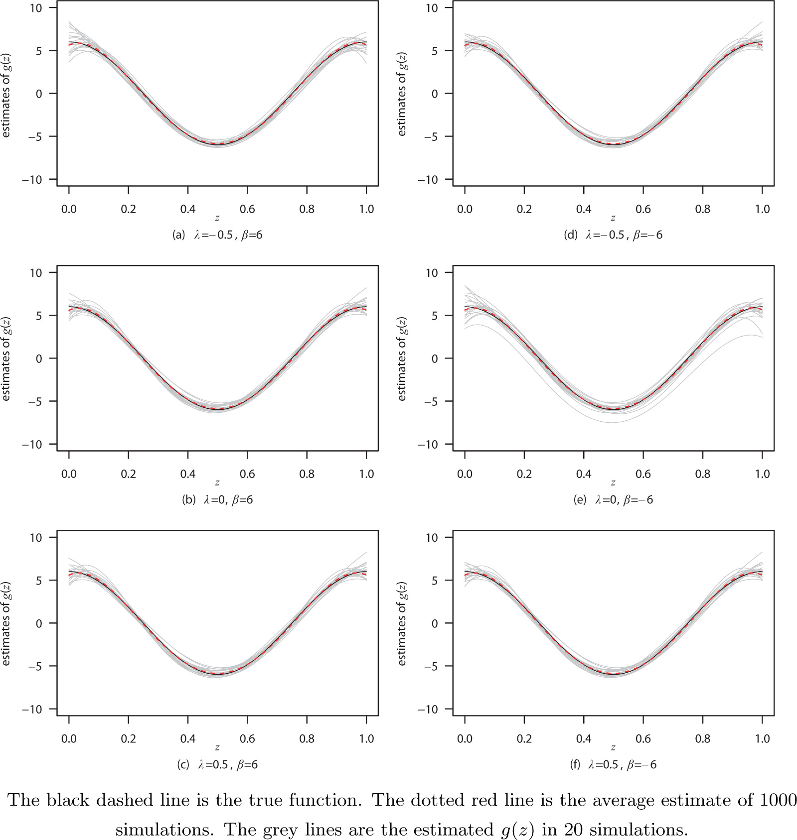
The plots of the estimates of g(z) = 6cos(2πz) under model (8) with n = 200 and σ = 1 for different values of λ and β.

5 Appendix technicalities

We denote tr(A) = trace(A) for a square matrix A.

Before we prove the main results, we first give some useful convergence results. By Assumption 3(i), we assume without loss of generality that: E {p_kK(zi)p_jK(zi)} = I_jk, where I_jk denotes the (j, k)th element of the identity matrix. Let ||·|| denotes the Euclidean norm. Denote Q=P′Pn, we obtain

Let 1_n denote the indicator function for the smallest eigenvalue of Q being greater than 1/2. Then limn→∞P(1n=1)=1. By Assumption 1, we obtain

and

6 Acknowledgements

We thank the referees for their time and comments.

References

[1] Cliff A D, Ord J K. Spatial autocorrelation. London: Pion Ltd, 1973.Search in Google Scholar
[2] Anselin L. Spatial econometrics: Methods and models. The Netherlands: Kluwer Academic Publishers, 1988.10.1007/978-94-015-7799-1Search in Google Scholar
[3] Cressie N. Statistics for spatial data. JohnWiley Sons, New York, 1993.10.1002/9781119115151Search in Google Scholar
[4] Anselin L, Bera A K. Spatial dependence in linear regressionmodels with an introduction to spatial econometrics. In: Ullah A, Giles D E A. Handbook of Applied Economics Statistics. Marcel Dekker, New York, 2002.Search in Google Scholar
[5] Ord J K. Estimation methods for models of spatial interaction. Journal of the American Statistical Association, 1975, 70: 120–126.10.1080/01621459.1975.10480272Search in Google Scholar
[6] Smirnov O, Anselin L. Fast maximum likelihood estimation of very large spatial autoregressive models: A characteristic polynomial approach. Computational Statistics and Data Analysis, 2001, 35: 301–319.10.1016/S0167-9473(00)00018-9Search in Google Scholar
[7] Kelejian H H, Prucha I R. A generalized spatial two-stage least squares procedure for estimating a spatial autoregressive model with sutoregressive disturbance. Journal of Real Estate Finance and Economics, 1998, 17: 99–121.10.1023/A:1007707430416Search in Google Scholar
[8] Kelejian H H, Prucha I R. A generalized moments estimator for the autoregressive parameter in a spatial model. International Economic Review, 1999, 40: 509–533.10.1111/1468-2354.00027Search in Google Scholar
[9] Kelejian H H, Prucha I R. Specification and estimation of spatial autoregres-sive models with autoregressive and heteroskedastic disturbances. Journal of Econometrics, 2010, 157: 53–67.10.1016/j.jeconom.2009.10.025Search in Google Scholar PubMed PubMed Central
[10] Lee L F. Asymptotic distribution of quasi-maximum likelihood estimators for spatial autoregressive models. Econometrica 2004, 72: 1899–1925.10.1111/j.1468-0262.2004.00558.xSearch in Google Scholar
[11] Su L, Jin S. Profile quasi-maximum likelihood estimation of spatial autoregressive models. Journal of Econometrics, 2010, 157: 18–33.10.1016/j.jeconom.2009.10.033Search in Google Scholar
[12] Lin X, Lee L F. GMM estimation of spatial autoregressive models with unknown heteroskedasticity. Journal of Econometrics, 2010, 157(1): 34–52.10.1016/j.jeconom.2009.10.035Search in Google Scholar
[13] Su L. Semi-parametric GMM estimation of spatial autoregressive models. Journal of Econometrics, 2012, 167: 543–560.10.1016/j.jeconom.2011.09.034Search in Google Scholar
[14] Ai C, Chen X. Efficient estimation of models with conditional moment restrictions containing unknown functions. Econometrica 2003, 71: 1795–1843.10.1111/1468-0262.00470Search in Google Scholar
[15] Newey W K. Convergence rates and asymptotic normality for series estimators. Journal of Econometrics, 1997, 79: 147–168.10.1016/S0304-4076(97)00011-0Search in Google Scholar
[16] Lee L F. GMM and 2SLS estimation of mixed regressive, spatial autoregressive models. Journal of Econometrics, 2007, 137: 489–514.10.1016/j.jeconom.2005.10.004Search in Google Scholar
[17] Case A C. Spatial patterns in household demand. Econometrica, 1991, 59: 953–965.10.2307/2938168Search in Google Scholar
© 2014 Walter de Gruyter GmbH, Berlin/Boston
Articles in the same Issue
- Forecasting the Crude Oil Price with Extreme Values
- Pricing Strategy and Governments Intervention for Green Supply Chain with Strategic Customer Behavior
- Fiscal Behavior Volatility, Economic Growth, and Urban-Rural Income Disparity