Price Increasing Timing of Competitive Perishable Products
-
Wensi Zhang
 ,
Jinlin Li
,
Jinlin Li

Abstract
Dynamic pricing has been proven to be an effective tool to increase revenue in many industries. We discuss the optimal time point to increase price of perishable products under duopoly competition in revenue management. We propose a game-theoretic model to describe the price increasing timing problem of competitive perishable products in the same market. By solving this problem, we show the existence of Stackelberg equilibrium point and Cournot equilibrium point when choosing the optimal price switching time. To illustrate our results, we also present a numerical example. Our results are applicable for decision makers to determine the optimal time to stop discounting.
1 Introduction
Revenue management problem can be described as “selling the right product to the right customer at the right time” (see Bitran and Caldentey[1]), from this aspect it is important for decision makers to determine the product price in real-time to maximize revenue. Dynamic pricing is a strategy that firms change their prices during the selling horizon in response to changing consumer characteristics and competitors’ actions[2]. Dynamic pricing has been widely used in the industries whose products are perishable, i.e. the unsold products have little salvage value; the inventory cannot be replenished.
Many firms face the problem of determining price when the demand not only depends on their own prices, but also depends on the prices of competitors. For perishable products, the following two cases are very common: For the first case, for instance, fashion dresses, the initial prices are always very high; however, when the selling season passes, the prices will be lower because the unsold products have little salvage value. For the second case, for instance, airline and hotel industry, the earlier you book the ticket or the room, the lower price you will pay. The sellers have incentive to increase the price if the sale goes well initially in order to reserve products for potential later customers who may be willing to pay higher price. Take airline flight for example, when it is near to the takeoff time, the price of the ticket may have no discount. It is important for the airline firms to decide when to start marking up price, without stopping discounting so early that the high price may alienate customers, or so late that the firms cannot get enough revenue.
Dynamic pricing problems have been studied extensively in revenue management literatures. Gallego and Van Ryzin[3] investigate the dynamic pricing problem when demand is price sensitive and use a heuristic algorithm to find out the optimal pricing policy. They also propose the two-fare policy in airline industry. Feng and Xiao[4] study a continuous-time RM model with reversible price and show that a subset of the prices that form a concave envelope is potentially optimal. Gallego and Van Ryzin[5] consider overbooking and no-show into the airline dynamic pricing model. In addition, dynamic pricing also has been studied in many other fields to maximize revenue. Aziz et al.[6] propose a hotel revenue management model based on dynamic pricing to maximize the revenue of the room. Tang et al.[7] investigate the optimal price and ordering decisions of newsvendor problem under random demands with a dynamic pricing policy. However, most of these studies focused on monopolistic models and ignored the fact that the substitutable products provided by different sellers.
Recently, more and more literatures about dynamic pricing problem consider the competition between firms. Dasci[8] uses a two-period model to analyze the dynamic pricing behavior of two firms that have substitutable products. Netessine and Shumsky[9] concern the seat inventory control problem under both horizontal competition and vertical competition and provide a pure-strategy Nash equilibrium. Gallego et al.[10] show the existence of unique Nash equilibrium in a Bertrand oligopoly price competition game using a possibly asymmetric attraction demand model. Dong et al.[11] consider the dynamic pricing model and inventory control of substitute products. Mak et al.[12] propose an equilibrium model of duopolistic pricing with alternating offers while Martínez-de-Albéniz and Talluri[13] discuss price competition for an oligopoly in a dynamic setting. The both two researches assume that each seller has fixed inventory and the selling horizon is finite. Nowadays, many studies focus on the customer choice when consider dynamic pricing problem under competition (Lin and Sibdari[14]; Zhang and Cooper[15]; Akçay et al.[16]). Most of these articles are analyzed from the aspect of setting different prices at different time.
To the best of our knowledge, there are limited literatures considering about when to start increasing or decreasing price. Gallego and Van Ryzin[3] first propose the concept of “stopping time”, and give the best time to switch the price. Feng and Gallego[17] address the problem of deciding the optimal timing of a single price change from a given initial price to either a given lower or higher second price, and show the optimality of threshold policies. However, the background of the both two literatures is monopoly market. Yang and Zhou[18–19] investigate the Cournot equilibrium point and Stackelberg equilibrium point of the price decreasing time of two competitive perishable products respectively.
In this paper, we discuss the optimal price increasing time of competitive perishable products, which is widely used in airline industry; and familiar with Yang and Zhou[18–19], we find the Cournot equilibrium point and Stackelberg equilibrium point. At last, we provide a numerical example in airline industry to illustrate our results.
2 Model description
We assume that there are two firms (firm 1 and firm 2) selling two competitive and substitutable perishable products in the same market over a finite selling horizon [0, T]. Each product has initial inventory Ni (i = 1, 2). The whole selling season can be divided into two periods, and firms will choose the optimal time ti to switch their prices. This is a markup problem, which means the price in the first period is lower than in the second one. We define the price of product i in the first period by
Depending on the result of Gallego and Ryzin, under the condition that there is no competition, the optimal switch time of product i can be given by:
Assume that T10 < T20, i.e. if we don’t take the competition into consideration, the price increasing time point of product 1 is earlier than product 2.
To simplify the problem, we assume that when both the two products are sold at the lower price, the competition of the two firms can be neglected. However, when one product (assume product 1) increases its price, and the other one (product 2) still keeps the lower price, because of a smaller discount, an amount of customers of product 1 will turn to purchase product 2. Let ρ (0 < ρ < 1) be the transition probability, we can get the demands of the two products during different time intervals (see Figure 1).
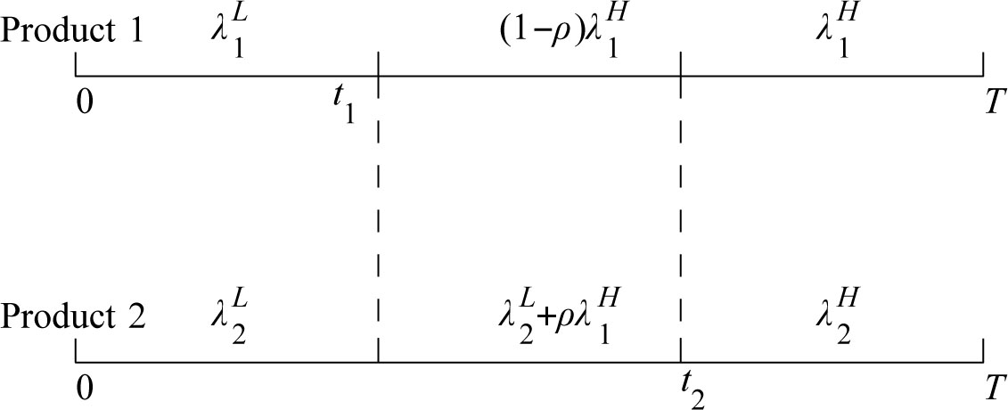
Distribution of demands when t1 < t2
3 Stackelberg equilibrium point of price increasing time
To simplify the model, we assume that in the leader-follower model, firm 1 acts as the leader and firm 2 acts as the follower. That means firm 2 always makes its decision to maximize its own revenue after observing the act of firm 1, so it is apparently that t1 < t2. The game rule can be described as: firm 1 chooses its time point t1 to increase the price of product 1, firm 2 chooses the optimal time t2 to maximize its revenue J2; firm 1 gets the feedback information of firm 2 and can maximize the revenue of product 1 by setting t1 properly.
As described in Section 2, with transition probability ρ, the revenue functions of product 1 and 2 can be written as:
Depends on the constraints of initial inventory and finite selling horizon, the strategy space can be determined by the following inequalities:
From these constraints, we can easily see that not only the revenue of each firm depends on its competitor’s strategy, but also their strategy spaces are not independent from each other. In addition, we can see all the constraints (4)–(6) are linear constraints, so we can solve this problem by the graphic method to find out their Stackelberg equilibrium point.
From inequalities (4) and (5) we can get:
In Figure 2, the shaded part denotes the strategy space of t1 and t2 formed by inequalities (4)–(6). Because
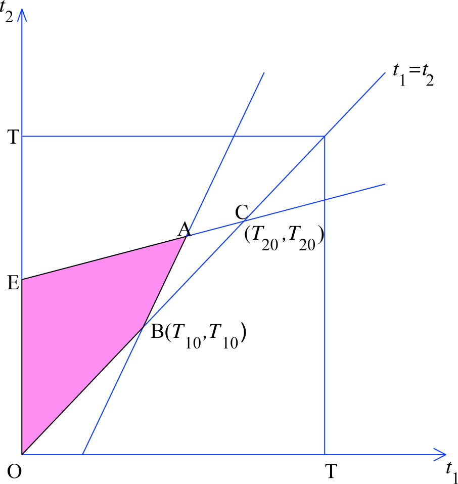
Strategy space when t1 < t2
Proposition 1
(T1, T2) is the Stackelberg equilibrium point.
Proof
Assume that product 1 increases its price at t1, we optimize the revenue of firm 2, i.e. J2. Transform equation (3):
Because higher price will bring lower revenue, we know that
Then, we will consider the strategy of product 1. If we choose strategy from segment AE, J1 can be rewritten as
We’ve already known
Till now, we prove that (T1, T2) is the Stackelberg equilibrium point.
4 Cournot equilibrium point of price increasing time
In this section, we consider a more common case: the two firms make decision to increase price simultaneously. We still assume that T10 < T20 here. When there exists competition between the two firms, the order of price increasing time point may change. The first case is t1 < t2, the demands of the two products can be found in Figure 1. The other case is t1 ≥ t2, the demands of the two products can be described by Figure 3. Here we assume the transition probability is ρ′.
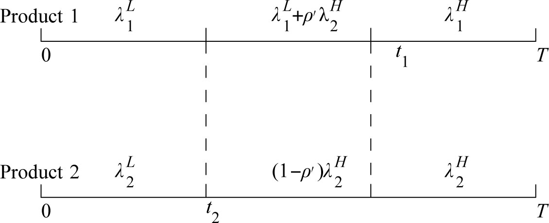
Distribution of demands when t1≥ t2
In the first case (t1 < t2), the revenue functions and strategy space can be described by (2)∼(6). In the second case (t1 ≥ t2), the revenue functions of product 1 and 2 can be written as
Depends on the constraints of initial inventory and finite selling horizon, the strategy space can be decided by the following conditions.
We can give another form of
We see that
The revenue functions and strategy space of the two products in the first case is the same with what we discuss in Section 3. However, the method to solve this problem is different from that in Section 3. In Figure 2, when t2 is fixed, t1 takes value in segment OB and segment AB; when t1 is fixed, t2 takes value in segment AE. Their intersection point is A, so (T1, T2) is the Cournot equilibrium point.
In the second case (t1 ≥ t2), we can get the strategy space of the two firms in Figure 4. When t1 is fixed, t2 will take value in segment OB, and when t2 is fixed, t1 will take value in segment DB. So point B(T10, T10) is Cournot equilibrium point.
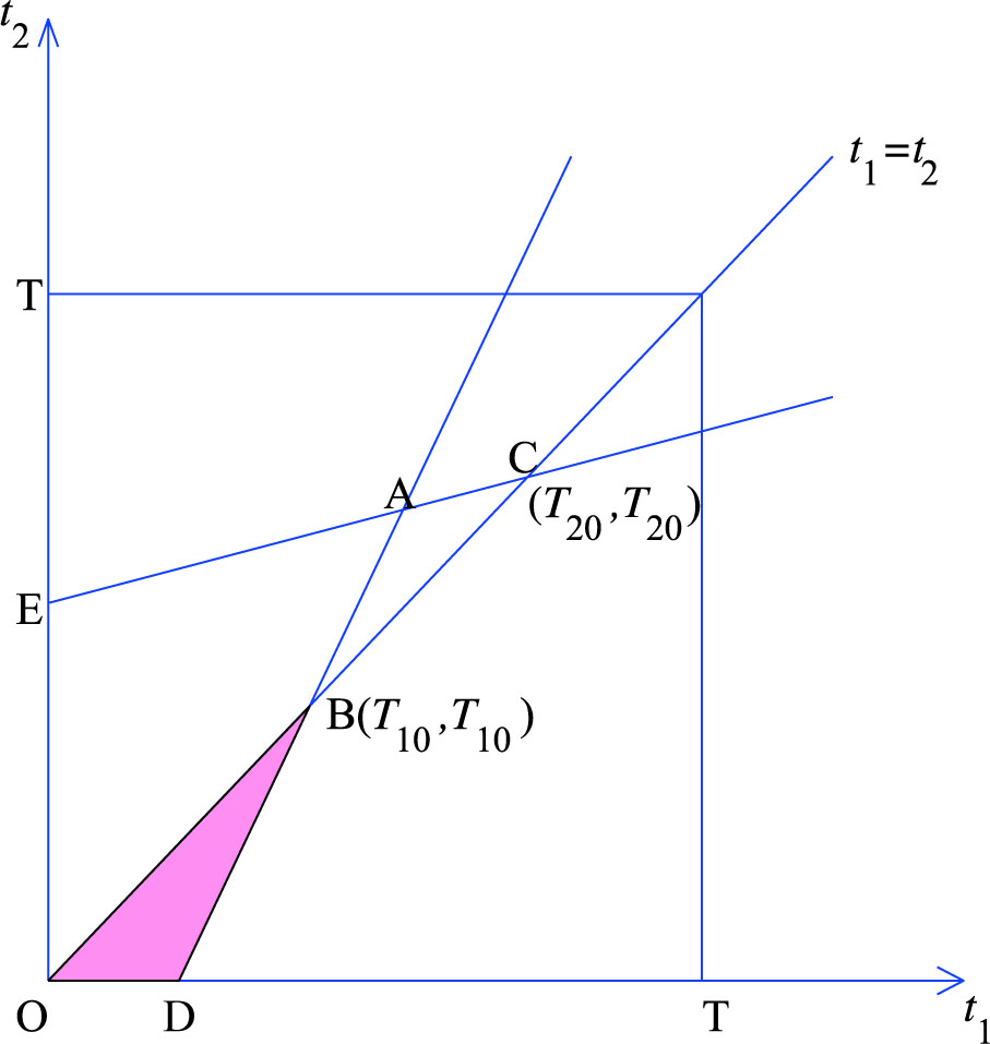
Strategy space when t1≥ t2
As we have analyzed above, in the first case, firm 1 will increase the price of product 1 at T1 while firm 2 will increase price at T2. This result coincides with Stackelberg equilibrium. However, in the second case, both firm 1 and firm 2 will increase the prices of their products at T10. Then, will the both two equilibrium outcomes be reality? For product 2, according to our calculation, when it increases price at T2 in the first case, firm 2 will get more revenue than its monopoly revenue. In the second case, if the two products increase prices simultaneously, that means there is no transition of customers between the two firms. So firm 2 prefers the first Cournot equilibrium result to the second result. When time reaches the point T10, firm 2 will not increase its price; they will choose to wait for lager revenue; if firm 1 increases price while firm 2 keeps the lower price at this time, according to our analysis, the revenue of firm 1 will decrease. With this background, firm 1 will choose T1 to increase price to minimize its loss and firm 2 will then decide to increase its price at T2 to maximize its revenue. Thus we can get the following proposition:
Proposition 2
(T1, T2) is the Cournot equilibrium point.
5 Numerical example
In this section, we describe a numerical example to illustrate our result.
Assume that there are two competitive airline firms in the market, and both of them provide a flight between a typical origin-destination pair. Also, the two flights have the same leaving time. Each flight has 160 seats, i.e. N1 = N2 = 160. And the selling horizon T = 20, that means both the two firms begin to sell the tickets 20 days before the leaving time. We take the service quality, brand image and other factors into consideration, and give these following parameters:
Using (1) we calculate that T10 = 12, T20 = 16; and the monopoly revenue of each product: J10 = 1120, J20 = 848. Assuming that when firm 1 increases its price, the transition probability from firm 1 to firm 2 is ρ (0 < ρ < 1). Moreover, we can get
We list Ti and Ji when ρ takes different values in interval (0, T).
The impact of ρ on equilibrium result
| ρ | T1 | T2 | J1 | J2 |
|---|---|---|---|---|
| 0.1 | 12.33 | 15.67 | 1106.7 | 825 |
| 0.2 | 12.57 | 15.43 | 1097.1 | 854.8 |
| 0.3 | 12.75 | 15.25 | 1090 | 857 |
| 0.5 | 13 | 15 | 1080 | 860 |
| 0.7 | 13.17 | 14.83 | 1073.3 | 862 |
| 0.9 | 13.28 | 14.71 | 1068.6 | 863.4 |
From this table we can see that the competition will decrease firm 1’s revenue while increase the revenue of firm 2. What’s more, the larger transition probability ρ is, the later will firm 1 increase its price and the earlier will firm 2 change its price; and accordingly, the more revenue firm 2 gets, and the more loss will firm 1 suffer.
This result illustrates that when a competitor enters a market, it is certain that the competitor will seize market share of the monopoly company. In most Stackelberg equilibrium problems, the leader can get more revenue than when it is monopoly; however, when we consider the price increasing timing problem, the result may be different. It is reasonable because if the new comer of the market puts off its price increasing time point, the leader of the market will face the loss of run off of customer. So the optimal choice of the leader is to postpone its price increasing time point. Moreover, because increase price brings the transition of customers, the first mover of the market will get less revenue than the case that there is no competition.
6 Conclusion
In this paper, we propose a game-theoretic model to describe the price increasing timing problem of competitive perishable products. By solving this problem, we find the Stackelberg equilibrium point and Cournot equilibrium point of the optimal price switching time. In Cournot game, though the two competitors make decision simultaneously, it still gets the same result with Stackelberg game. Firm 1 will postpone its price increasing time to decrease the loss caused by competition. This paper is helpful for service process design and operation because for many industries that provide perishable products, like airline and hotel industry, it is important for decision makers to choose the optimal time to switch their prices, avoiding changing prices so early that may alienate customers, or so late that causes low revenue. What’s more, it is useful for customers when they book a airline ticket or a room. Customers can choose their booking time depends on the price switching time point to maximize their utility. The results can lead to form a more efficient serve mechanism in perishable products selling.
There are several possible future research directions. First, customer choice model can be taken into account when analyze the transition probability. Second, we consider this problem under the two-class fare condition, the model can be extended to multi-class fare and consider more complicated situations. And furthermore, another extension would be incorporating oligopoly competition into our pricing model.
Acknowledgements
The authors thank Junli Lei and Yanhui Wang for their helpful comments and suggestions.
References
[1] Bitran G, Caldentey R. An overview of pricing models for revenue management. Manufacturing & Service Operations Management, 2003, 5(3): 203–229.10.1287/msom.5.3.203.16031Search in Google Scholar
[2] Talluri K T, Van Ryzin G J. The theory and practice of revenue management. Springer, 2005.10.1007/b139000Search in Google Scholar
[3] Gallego G, Van Ryzin G. Optimal dynamic pricing of inventories with stochastic demand over finite horizons. Management Science, 1994, 40(8): 999–1020.10.1287/mnsc.40.8.999Search in Google Scholar
[4] Feng Y, Xiao B. A continuous-time yield management model with multiple prices and reversible price changes. Management Science, 2000, 46(5): 644–657.10.1287/mnsc.46.5.644.12050Search in Google Scholar
[5] Gallego G, Van Ryzin G J. A multi-product, multi-resource pricing problem and its applications to network yield management. Operations Research, 1997, 45: 24–41.10.1287/opre.45.1.24Search in Google Scholar
[6] Aziz H A, Saleh M, Rasmy M H, et al. Dynamic room pricing model for hotel revenue management systems. Egyptian Informatics Journal, 2011, 12(3): 177–183.10.1016/j.eij.2011.08.001Search in Google Scholar
[7] Tang O, Nurmaya Musa S, Li J. Dynamic pricing in the newsvendor problem with yield risks. International Journal of Production Economics, 2012, 139(1): 127–134.10.1016/j.ijpe.2011.01.018Search in Google Scholar
[8] Dasci A. Dynamic pricing of perishable assets under competition: A two-period model. Faculty of Commerce, University of British Columbia November, 2003.Search in Google Scholar
[9] Netessine S, Shumsky R A. Revenue management games: Horizontal and vertical competition. Management Science, 2005, 51(5): 813–831.10.1287/mnsc.1040.0356Search in Google Scholar
[10] Gallego G, Huh W T, Kang W, et al. Price competition with the attraction demand model: Existence of unique equilibrium and its stability. Manufacturing & Service Operations Management, 2006, 8(4): 359–375.10.1287/msom.1060.0115Search in Google Scholar
[11] Dong L, Kouvelis P, Tian Z. Dynamic pricing and inventory control of substitute products. Manufacturing & Service Operations Management, 2009, 11(2): 317–339.10.1287/msom.1080.0221Search in Google Scholar
[12] Mak V, Rapoport A, Gisches E J. Competitive dynamic pricing with alternating offers: Theory and experiment. Games and Economic Behavior, 2012, 75(1): 250–264.10.1016/j.geb.2011.08.018Search in Google Scholar
[13] Martínez-de-Albéniz V, Talluri K. Dynamic price competition with fixed capacities. Management Science, 2011, 57(6): 1078–1093.10.1287/mnsc.1110.1337Search in Google Scholar
[14] Lin K Y, Sibdari S Y. Dynamic price competition with discrete customer choices. European Journal of Operational Research, 2009, 197(3): 969–980.10.1016/j.ejor.2007.12.040Search in Google Scholar
[15] Zhang D, Cooper W L. Pricing substitutable flights in airline revenue management. European Journal of Operational Research, 2009, 197(3): 848–861.10.1016/j.ejor.2006.10.067Search in Google Scholar
[16] Akçay Y, Natarajan H P, Xu S H. Joint dynamic pricing of multiple perishable products under consumer choice. Management Science, 2010, 56(8): 1345–1361.10.1287/mnsc.1100.1178Search in Google Scholar
[17] Feng Y, Gallego G. Optimal starting times for end-of-season sales and optimal stopping times for promotional fares. Management Science, 1995, 41(8): 1371–1391.10.1287/mnsc.41.8.1371Search in Google Scholar
[18] Yang H, Zhou J. A Cournot game of setting optimal markdown timing for perishable products. Chinese Journal of Management Science, 2006, 14(3): 45–50.Search in Google Scholar
[19] Yang H, Zhou J. A Stackelberg game of setting optimal markdown timing for perishable products. Journal of Industrial Engineering/Engineering Management, 2007, 21(3): 155–158.Search in Google Scholar
© 2014 Walter de Gruyter GmbH, Berlin/Boston
Articles in the same Issue
- A Study on the Chinese Enterprise Annuity Replacement Rate Problem
- A Novel Intelligence Recommendation Model for Insurance Products with Consumer Segmentation
- Price Increasing Timing of Competitive Perishable Products
- Modeling and Forecasting Morbidity and Disease-mortality of Chinese Impaired Lives with the General Chronic Diseases
- A Dynamic Model of Housing Wealth Effect: Based on the Diversity of Wealth Expectations
- Well-posedness and Stability of the Repairable System with Three Units and Vacation
- Bayesian Subset Selection for Reproductive Dispersion Linear Models
- Study on Evolutionary Algorithm Online Performance Evaluation Visualization Based on Python Programming Language