Statistical regimes of electromagnetic wave propagation in randomly time-varying media

1 Introduction

Wave propagation in time-varying media has emerged as a fertile ground for uncovering fundamentally new physical phenomena that are unattainable in static or spatially inhomogeneous systems [1], [2], [3], [4], [5], [6]. In contrast to stationary media, where energy is conserved, time-dependent systems break energy conservation due to the explicit temporal variation of material parameters. This leads to unconventional scattering dynamics, temporal energy amplification, and novel mechanisms for controlling wave transport. Such effects are increasingly relevant in modern optics, materials science, and communication technologies, where temporal modulation enables dynamic functionalities beyond the capabilities of static systems.

Recent advances have revealed a variety of phenomena unique to time-varying systems, including temporal photonic crystals, momentum band gaps, temporal Brewster effects, temporal holography, and ultrafast wave steering [7], [8], [9], [10], [11], [12], [13], [14], [15], [16], [17], [18], [19], [20], [21], [22]. Among these, temporal disorder – random fluctuations in material properties over time – has drawn particular attention for its striking analogy to Anderson localization in spatially disordered media [23], [24], [25], [26], [27], [28], [29], [30]. Temporal disorder can induce strong localization effects, leading to suppression of wave propagation. These effects are of both fundamental interest and practical importance, with potential applications in ultrafast switching, energy harvesting, and temporally gated information processing.

Despite growing interest, the statistical behavior of waves in randomly time-varying media remains incompletely understood. Previous studies suggest that energy distributions may evolve from negative exponential forms at short times to log-normal distributions at longer times [24]. However, key questions remain unresolved: What governs the transition between these regimes? Is log-normal behavior truly universal? And how do initial wave conditions influence the statistical evolution?

In this work, we present a comprehensive analytical and numerical study of electromagnetic wave propagation in isotropic, spatially uniform media with randomly time-varying permittivity. Using the invariant imbedding method (IIM) [30], [31], [32], [33], [34], [35], [36], [37], [38], we derive exact moment equations for reflectance, transmittance, and total energy density. For unidirectional input, our analysis reveals three distinct statistical regimes: gamma-distributed energy at early times, negative exponential behavior at intermediate times, and a quasi-log-normal distribution at long times, which is mathematically distinct from the true log-normal. In contrast, symmetric bidirectional input produces genuine log-normal statistics across all time scales.

These findings are supported by extensive calculations based on two complementary disorder models: delta-correlated Gaussian noise and piecewise-constant stepwise fluctuations. Both models confirm that wave statistics are highly sensitive to the initial input symmetry and the duration of temporal disorder. Our results establish a unified framework for understanding statistical fluctuations and localization phenomena in time-varying systems and provide practical guidance for the design of dynamically tunable photonic and electromagnetic devices.

2 Theory

We investigate electromagnetic wave propagation in an isotropic, spatially uniform medium with time-dependent properties. The electric displacement field D satisfies the wave equation

where ϵ and μ are the permittivity and permeability, respectively, c is the speed of light in vacuum, and k is the constant wavenumber. We consider wave propagation along the x axis.

In a time-independent medium, the field components evolve as exp[i(kx ∓ ωt)]. When material parameters vary with time, scattering occurs at temporal interfaces, generating reflected and transmitted components. We consider a unit-amplitude plane wave initially propagating in the +x direction. If ϵ and μ vary only within the interval 0 ≤ t ≤ T, the displacement field is given by

where ω 1 = ω 0 / ϵ 1 μ 1 and ω 2 = ω 0 / ϵ 2 μ 2 , with ϵ _1,2 and μ _1,2 denoting the permittivity and permeability before and after the modulation, respectively. All parameters are assumed to be positive. The coefficients s(T) and r(T) represent the temporal transmission and reflection amplitudes.

We analyze this system using the IIM [30], [31], [32], [33], [34], [35], [36], [37], [38], a powerful tool originally developed for spatially inhomogeneous systems. In the IIM, the independent variable is not time t itself but the modulation interval T. The method transforms the boundary value problem into an initial value problem, yielding coupled differential equations for r and s with respect to the imbedding parameter τ ∈ [0, T], which serves as the running duration of temporal variation:

where

and n 2 = ϵ 2 μ 2 . The initial conditions at τ = 0, corresponding to a sudden temporal interface, are given by

From Eq. (3), it follows that the difference between the squared magnitudes of the transmission and reflection amplitudes remains invariant during the temporal modulation:

We define the temporal transmittance S and reflectance R as

It immediately follows that S − R = 1 for arbitrary temporal variations of ϵ and μ. Since both S and R are nonnegative, we always have S ≥ 1, indicating that total temporal reflection is not possible in isotropic media. In the special case of perfect transmission (R = 0), we find S = 1, implying no amplification.

In Eq. (2), s and r are defined relative to the displacement field D of the initial wave. The energy density is |D|²/(2ϵ) and the photon energy is ℏ ω = ℏ c k / ϵ μ , giving a photon number density

Thus, the definitions of S and R in Eq. (7) correspond to the ratios of photon number densities in the transmitted and reflected waves to that of the initial wave.

After temporal scattering, equal numbers of forward- and backward-moving photons are created or annihilated. The forward photon carries momentum +ℏk and the backward photon −ℏk, so the total momentum density relative to the initial wave is ℏk(S − R), which remains constant. The relation S − R = 1 thus directly reflects momentum conservation.

Alternatively, transmittance and reflectance may be defined in terms of the energy flux, given by the product of the energy density and the wave velocity:

In this formulation, S _E − R _E is generally not conserved, except in the special case ϵ ₁ μ ₁ = ϵ ₂ μ ₂, for which S = S _E and R = R _E .

In this study, we examine electromagnetic wave propagation in media where the dielectric permittivity ϵ(t) varies randomly in time. Although our method can be readily extended to cases where both ϵ and μ fluctuate stochastically, we fix μ = 1 throughout this work for simplicity. Two stochastic models are considered. Model 1 assumes delta-correlated Gaussian noise:

where ϵ ̄ is the mean permittivity and g ₀ (with units of time) quantifies the disorder strength. This model is analytically tractable and enables semi-analytical evaluation of all disorder-averaged moments. Although ϵ(t) may temporarily take negative values in this model, it does not produce any distinctive effects in the weak-disorder cases considered in the present work. Model 2 describes piecewise-constant disorder: the fluctuation δϵ is constant within each time interval of duration Λ, and is abruptly updated at the end of each interval. Each new value is drawn independently from a uniform distribution over [−a ₀, a ₀]. The process continues over a total duration T. This model is particularly well suited for computing statistical quantities that are difficult to evaluate using Model 1, such as the moments of the logarithm of the wave energy and the full probability distributions of the logarithms of both the reflectance and the wave energy.

In Model 1, we study the stochastic differential equation (Eq. (3)) with random coefficients proportional to 1/ϵ. For a random function in the denominator, we assume weak disorder and expand the inverse permittivity as

Alternatively, ϵ may be modeled as a dichotomous random variable; in this case, even for strong disorder, the disorder average can be performed exactly using the Shapiro–Loginov formula of differentiation [39].

Our goal is to compute the statistical moments of the transmittance, reflectance, and total wave energy density. To this end, we define the moment function Z abcd = r a r * b s c s * d , where a, b, c, d = 0, 1, 2, ⋯. Applying Eq. (3) together with the Furutsu–Novikov formula [40], [41], we derive the following evolution equation for Z _abcd :

where the coefficients are given by

The auxiliary parameters are defined as

The IIM can be extended to more general cases in which plane waves with arbitrary relative amplitudes propagate simultaneously in opposite directions at the initial time. In this case, we generalize Eq. (2) and the initial conditions in Eq. (5) as follows:

where v and w denote the amplitudes of the incident waves propagating in the +x and −x directions, respectively, for t < 0. Under these generalized initial conditions, the invariant imbedding equations in Eqs. (3) and (12) remain valid and unchanged.

The IIM can be viewed as a continuum generalization of the transfer matrix method widely used in wave propagation studies and offers several advantages over alternative approaches. First, for temporal variations described by continuous or piecewise continuous functions, the invariant imbedding equations can be integrated directly using standard differential equation solvers, eliminating the need for artificial discretization. Second, for random temporal variations, the method can incorporate stochastic calculus tools – such as the Furutsu–Novikov formula or the Shapiro–Loginov formula of differentiation – to perform analytical disorder averaging, as shown in the derivation of Eq. (12). This transforms the original equations with random coefficients into a larger set of coupled equations with deterministic coefficients, enabling direct solutions without numerical averaging over many realizations. This often results in substantial computational efficiency and, in some cases, allows for closed-form analytical solutions [38]. Third, in nonlinear systems, the formalism introduces an additional invariant imbedding equation for the wave intensity, which naturally captures nonlinear effects such as bistability and multistability and enhances the efficiency of both analytical and numerical treatments [34], [35], [36].

3 Results

We present the results of our analytical and numerical calculations. For simplicity, we focus on Model 1 with ϵ 1 = ϵ 2 = ϵ ̄ = 1 and μ ₁ = μ ₂ = μ = 1, under which the parameters in Eq. (14) simplify to α ̄ = 0 , β ̄ = 1 , and γ = 1/2. In this case, the reflectance and transmittance reduce to R = |r|² and S = |s|², respectively.

The structure of Eq. (12) couples each moment Z _abcd to others with the same total indices, satisfying a′ + c′ = a + c and b′ + d′ = b + d. To compute Z _nn00 = ⟨R ⁿ ⟩ and Z _00nn = ⟨S ⁿ ⟩, it suffices to solve a finite system of (n + 1)² coupled first-order differential equations for the moments Z _{i,j,n−i,n−j} , where i, j = 0, 1, …, n. Since the coefficients in these equations are constant, they are, in principle, analytically solvable; however, explicit solutions are generally intractable. We therefore obtain numerically precise values of ⟨R ⁿ ⟩ and ⟨S ⁿ ⟩ by solving the (n + 1)² coupled equations derived from Eq. (12) using a Fortran-based code combined with IMSL library routines developed by the authors.

When ϵ ₁ = ϵ ₂ and μ ₁ = μ ₂, the quantities R and S represent not only the photon number densities but also the reflected and transmitted energy densities, respectively, normalized to that of the initial wave. As seen from Eq. (2), the total energy density relative to the initial wave for t > T, denoted U, is given by U = R + S = 2R + 1. This expression follows from the standard practice in electromagnetic wave propagation of defining both energy density and energy flux as time-averaged quantities, particularly for monochromatic waves. The temporal evolution of statistical moments depends on the time regime – short, intermediate, or long. For studying early-time dynamics, reflectance is a more sensitive observable than total energy, since R(0) = 0 while U(0) = 1.

The evolution also depends on the initial wave conditions. In Figure 1, we plot the first four moments of the reflectance in the short-time regime, assuming the wave initially propagates only in the forward direction (i.e., r(0) = w = 0, s(0) = v = 1). The corresponding initial condition is Z _abcd (0) = 1 if a = b = 0, and zero otherwise.

Figure 1:

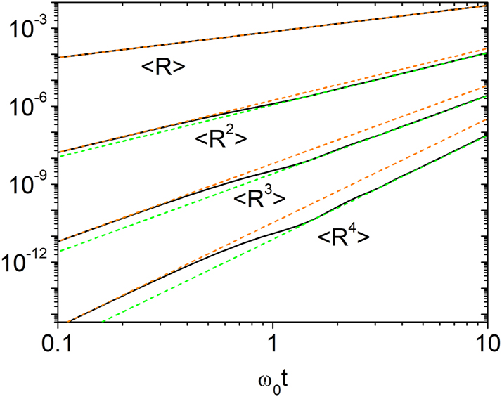
Log-log plot of the temporal evolution of the reflectance moments ⟨R⟩, ⟨R ²⟩, ⟨R ³⟩, and ⟨R ⁴⟩ for Model 1 with g = 0.003. Numerical results from Eq. (12) are shown as black solid lines. The orange dashed lines represent the short-time behavior predicted by Eq. (16), while the green dashed lines correspond to the intermediate-time behavior described by Eq. (17). For n ≥ 2, a clear crossover from the initial regime governed by Eq. (16) to the regime of Eq. (17) occurs near ω ₀ t ≈ 1.

We find that, at early times, the reflectance moments are

while for ω ₀ t ≈ 1 they cross over to

signaling a change in the underlying probability distribution. These behaviors are confirmed numerically and derived analytically in the Appendix. At early times, R follows a gamma distribution:

with moments

As ω ₀ t grows to order unity, this distribution transitions to a negative exponential form,

whose moments are given by Eq. (17). This regime persists up to ω ₀ t ≲ g ⁻¹.

Under the random phase approximation (RPA), which assumes

the reflectance moments exactly match those of the negative exponential distribution. This result, consistent with [24], confirms that under RPA, the reflectance indeed follows a negative exponential distribution.

In summary, in the intermediate regime 1 ≲ ω ₀ t ≲ g ⁻¹, the reflectance moments converge to those of a negative exponential distribution. The transition from gamma to negative exponential, occurring near ω ₀ t ∼ 1, is driven by complete randomization of the phases of r and s, and is largely insensitive to disorder strength in the weak-disorder regime. The crossover time is inversely proportional to ω ₀ = ck.

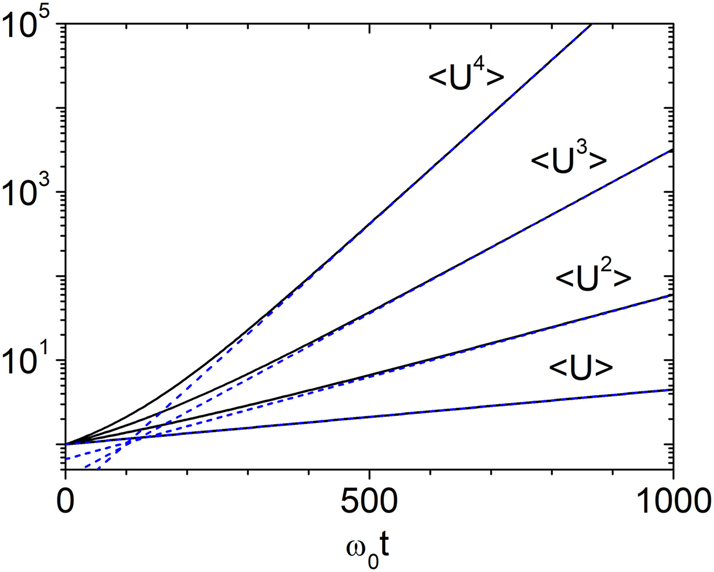
We now examine the time evolution of the total wave energy, focusing on the long-time regime. In Figure 2, we present the first four moments of U, which show excellent agreement with the analytical expression

valid over a broad temporal range, g ⁻¹ ≲ ω ₀ t ≲ 10⁶. The case n = 1 is special. Numerical results confirm that the average energy is accurately described by

throughout the entire interval 0 < ω ₀ t ≲ 10⁶.

Figure 2:

Temporal growth of energy moments for g = 0.003. The evolution of ⟨U⟩, ⟨U ²⟩, ⟨U ³⟩, and ⟨U ⁴⟩ is shown. Solid lines represent numerical results from Eq. (12), and dashed lines show the analytical prediction from Eq. (22). Excellent agreement is observed in the long-time regime ω ₀ t ≳ g ⁻¹.

Although Eq. (22) has the same exponential factor as the raw moments of a log-normal distribution,

the additional prefactor n!/(2n − 1)!! in Eq. (22) distinguishes the actual distribution from a true log-normal form. This prefactor modifies all moments, altering the peak position, width, and tail behavior of the probability density. While the two distributions become asymptotically similar as t → ∞, substantial and experimentally relevant deviations persist over a wide time range. We therefore classify the underlying statistics not as strictly log-normal, but as a quasi-log-normal distribution.

The exponential factor common to both forms can be obtained in a semi-analytical manner from Eq. (12). From full numerical solutions of Eq. (12), we find that, in calculating Z _nn00 = ⟨R ⁿ ⟩, all terms with a ≠ b or c ≠ d in Z _abcd decay rapidly at long times. This yields

where S = R + 1 and γ = 1/2. If we further incorporate the numerical observation that ⟨R ⁿ ⟩ increases rapidly with n in the long-time regime, we obtain

with τ replaced by t. This reasoning establishes the exponential scaling but not the numerical prefactor, which is governed by the evolution of the rapidly decaying terms in Eq. (12) and further constrained by the w/v ratio in Eq. (15), as discussed below.

In Figure 3, we plot the scaled energy moments

for n = 1, 2, 3, 4. In the long-time regime ω 0 t ≳ g − 1 , these values converge accurately to n!/(2n − 1)!! up to ω ₀ t ∼ 10⁶. Beyond this point, deviations emerge due to the rapid growth of ⟨U ⁿ ⟩ and the accumulation of numerical errors.

Figure 3:

Temporal variation of U _n for g = 0.003. Here, U n = ⟨ U n ⟩ exp − n ( n + 1 ) g ω 0 t / 4 . In the long-time regime, numerical results show excellent agreement with the analytical predictions from Eq. (22).

To characterize the reflectance distribution more precisely, we evaluate the dimensionless quantity

which eliminates time-dependent scaling and isolates the distribution’s intrinsic form. The value of F ₃ serves as a diagnostic: F ₃ = 5/9 ≈ 0.556 for a gamma distribution, 0.75 for a negative exponential, 1 for a log-normal, and 1.35 for the quasi-log-normal form given by Eq. (22). As shown in Figure 4, three distinct temporal regimes emerge: gamma-like for ω ₀ t ≲ 1, negative exponential for 1 ≲ ω ₀ t ≲ g ⁻¹, and quasi-log-normal for g ⁻¹ ≲ ω ₀ t ≲ 10⁶. Notably, F ₃ never reaches 1, indicating that R does not follow a true log-normal distribution. A similar trend is observed in the wave energy, with ⟨ U 3 ⟩ ⟨ U ⟩ 3 / ⟨ U 2 ⟩ 3 ≈ 1.35 at long times, consistent with quasi-log-normal statistics. Since g = g ₀ ω ₀, the crossover from negative exponential to quasi-log-normal behavior occurs at a time scale proportional to g 0 − 1 ω 0 − 2 .

Figure 4:

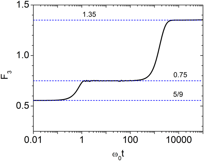
Temporal evolution of F ₃ for g = 0.003. F 3 ≡ ⟨ R 3 ⟩ ⟨ R ⟩ 3 / ⟨ R 2 ⟩ 3 evolves from an initial value of 5/9 (gamma distribution), passes through 0.75 (negative exponential distribution), and approaches 1.35, consistent with the quasi-log-normal form given in Eq. (22).

The statistical behavior is highly sensitive to the initial conditions. When waves initially propagate in both directions, the moments are determined by the initial condition Z abcd ( 0 ) = w a ( w * ) b v c ( v * ) d , with w and v defined in Eq. (15). The resulting statistics depend on the relative magnitudes of w and v. Figure 5 shows the scaled moments U _n (n = 1–5) as functions of R(0) = |w|² at ω ₀ t = 25,000, with S(0) = |v|² fixed at 1. As R(0) increases from 0 to 1 – corresponding to symmetric bidirectional wave input – all U _n increase and converge to 1. In this limit, the energy distribution becomes exactly log-normal, with U _n = 1 for all n.

Figure 5:

Scaled moments U _n /[1 + R(0)] ⁿ as functions of R(0) = |w|² for n = 1–5 at ω ₀ t = 25,000. S(0) = |v|² is fixed at 1.

This behavior is confirmed in Figure 6, which shows the first four moments of U for the symmetric case R(0) = S(0) = 1/2. The numerical results exhibit excellent agreement with the analytical prediction given by Eq. (24) at all times, confirming that the energy follows a log-normal distribution throughout the evolution.

Figure 6:

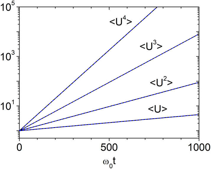
Temporal growth of energy moments for g = 0.003 with R(0) = S(0) = 1/2. Solid lines show numerical results from Eq. (12); dashed lines indicate the analytical prediction from Eq (24). The results confirm that the energy follows a log-normal distribution at all times when the initial waves propagate in opposite directions with equal amplitudes.

All numerical results in Figures 3–6 confirm that, in the long-time regime, the moments ⟨R ⁿ ⟩ and ⟨U ⁿ ⟩ follow the exponential scaling of Eq. (26). For ⟨U ⁿ ⟩, the prefactor is n!/(2n − 1)!! for unidirectional input and unity for symmetric bidirectional input. For more general initial conditions, the prefactor is expected to vary systematically with the ratio w/v. The observed trends – particularly the clear dependence on the initial condition in Figure 5 – provide strong evidence that this behavior persists in the infinite-time limit.

At this stage, it is instructive to compare our findings with those of ref. [24], which studied wave propagation in a spatially uniform, time-varying medium in the weak-disorder regime using the transfer matrix method. They reported that, in the time domain τ _m ≪ t ≪ τ _c , the wave energy follows a negative exponential distribution, whereas for t ≫ τ _c it follows a log-normal distribution. Our results for the intermediate-time regime (τ _m ≪ t ≪ τ _c ) are in excellent agreement with theirs. In our framework, the microscopic time τ _m corresponds to 1/ω ₀, and the crossover time τ _c to 1/(gω ₀). Their Fokker–Planck equation (Eq. (22)) contains the term z + z ² on the right-hand side. The negative exponential result in ref. [24] was obtained by neglecting the z ² term, while the log-normal result arose from neglecting the z term. From their definitions, z corresponds to our R and z + 1 to our S, so z + z ² maps directly to our RS. Neglecting the z ² term corresponds to the short-time regime, while neglecting the z term is equivalent to assuming R = S, i.e., identical propagation in both directions. Only in this latter limit does one recover a genuine log-normal distribution. Retaining both z and z ² terms naturally leads to a distribution distinct from the log-normal form.

We also remark on the scaling characteristics of the underlying probability distribution. In the long-time regime, it is governed by two parameters: gω ₀ t/4, which controls the exponential scaling of the moments, and the ratio w/v, which sets the time-independent prefactor. For fixed initial conditions, w/v is constant, leaving gω ₀ t/4 as the sole relevant parameter. In this qualified sense, the distribution exhibits single-parameter scaling [42], [43], although, as in conventional spatial localization, this behavior is expected to break down under strong disorder.

We further performed simulations using Model 2, where the random component δϵ remains constant over each time interval of duration Λ = 1/ω ₀ and is abruptly updated at the end of each interval. Each value is independently sampled from a uniform distribution over [−a ₀, a ₀], with a ₀ = 0.1. Since ϵ ̄ = 1 , ϵ(t) remains strictly positive within the range [0.9, 1.1]. Equation (3) was solved for 10⁶ independent realizations, and the results were ensemble averaged over the total duration T.

The average energy ⟨U⟩ grows exponentially at all times, regardless of the initial condition. Fitting this growth yields effective disorder strengths of g ≈ 0.00246 for unidirectional input and g ≈ 0.00242 for symmetric bidirectional input. Using these fitted values, we compared the numerical results from Model 2 with the analytical predictions of Eqs. (22) and (24). As shown in Figure 7(a), the energy moments for unidirectional input closely follow Eq. (22) in the long-time regime. For symmetric bidirectional input, the moments agree with the log-normal form of Eq. (24) at all times (Figure 7(b)). These results confirm that the statistical behavior is robust and essentially independent of the disorder model, provided the disorder is weak and short-range correlated.

Figure 7:

Temporal growth of energy moments under stepwise disorder (Model 2) with Λ = 1/ω ₀ and a ₀ = 0.1. Effective disorder strengths of g ≈ 0.00246 (unidirectional input) and g ≈ 0.00242 (symmetric bidirectional input) are obtained by fitting the exponential growth of ⟨U⟩. (a) Numerical results (solid lines) for unidirectional input [S(0) = 1, R(0) = 0] agree well with the analytical prediction from Eq. (22) (dashed lines) at long times. (b) For symmetric bidirectional input [S(0) = R(0) = 1/2], numerical results match the analytical expression from Eq. (24) at all times.

For Model 2 with Λ = 1/ω ₀ and a ₀ = 0.1, we also computed the mean and variance of ln U. Figure 8(a) and (b) show ⟨ ln U⟩, Var(ln U), and their ratio for unidirectional and symmetric bidirectional inputs. For symmetric input, the results agree with the log-normal predictions: ⟨ ln U⟩ = gω ₀ t/4, Var(ln U) = gω ₀ t/2, yielding a ratio of 2. In contrast, unidirectional input exhibits persistent deviations, with the ratio remaining well below 2 even at long times – indicating a clear departure from log-normal behavior.

Figure 8:

Temporal evolution of ⟨ ln U⟩, Var(ln U), and their ratio under stepwise disorder (Model 2) with Λ = 1/ω ₀ and a ₀ = 0.1. Results are averaged over 10⁶ random configurations. (a) Unidirectional input [S(0) = 1, R(0) = 0]. (b) Symmetric bidirectional input [S(0) = R(0) = 1/2] with effective disorder strength g ≈ 0.00242, showing rapid convergence to the log-normal value Var(ln U)/⟨ ln U⟩ = 2.

Finally, we computed the probability distributions of ln U and ln R using Model 2 under stepwise disorder with Λ = 1/ω ₀ and a ₀ = 0.1, based on 10⁶ independent simulations. Figure 9(a) and (b) show histogram-based probability density functions of ln U and ln R at various times for unidirectional input. Since U ≥ 1, ln U is always positive, while ln R spans the entire real axis. The distribution of ln U undergoes a clear crossover from an exponential-like form to a quasi-log-normal shape, while the distribution of ln R evolves from being highly skewed to increasingly symmetric over time. For symmetric bidirectional input (Figure 9(c)), the distribution of ln U remains Gaussian at all times, consistent with genuine log-normal behavior.

Figure 9:

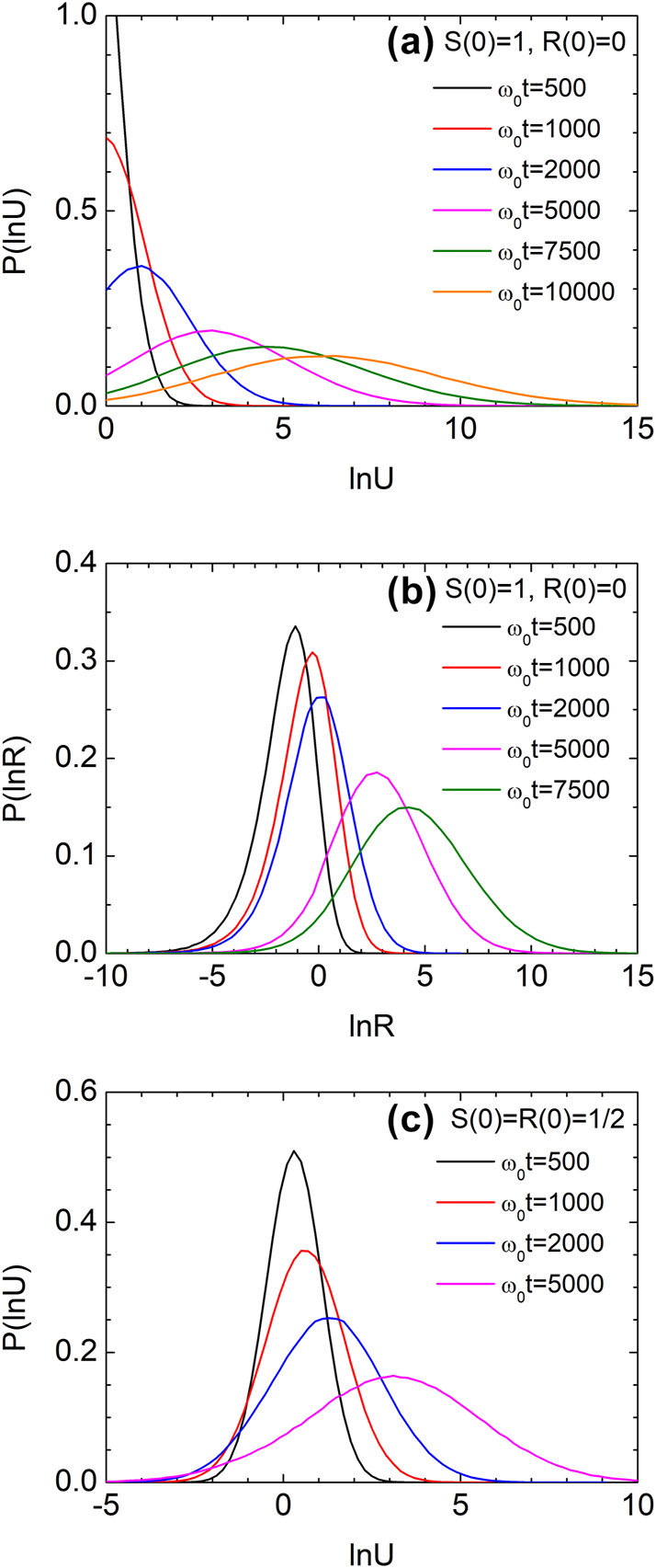
Evolution of probability density functions under stepwise disorder (Model 2) with a ₀ = 0.1 and Λ = 1/ω ₀. (a,b) Distributions of ln U and ln R for unidirectional input, obtained from histograms of 10⁶ samples at various times. (c) Distribution of ln U for symmetric bidirectional input, showing Gaussian behavior consistent with log-normal statistics.

4 Discussion

Our study shows that wave propagation in randomly time-varying media exhibits rich statistical behavior that differs fundamentally from that in spatially disordered systems. While earlier work characterized temporal Anderson localization in terms of negative exponential and log-normal statistics [24], we demonstrate that this picture is incomplete. In particular, the energy distribution is strongly influenced by the initial wave configuration – an effect largely overlooked in previous analyses.

For unidirectional input, the statistics evolve through three distinct regimes: a gamma distribution at early times, negative exponential behavior in the intermediate regime 1 ≲ ω 0 t ≲ g − 1 , and a quasi-log-normal distribution at long times. The latter deviates from a true log-normal form due to a distinct prefactor in the moments, originating from temporal interference and amplitude fluctuations. In contrast, symmetric bidirectional input yields genuine log-normal statistics across all time scales, as confirmed by analytical predictions, numerical simulations, and agreement in the scaled moments U _n and the ratio Var(ln U)/⟨ ln U⟩.

Momentum conservation plays a central role: although the total energy increases under temporal driving, the difference between reflected and transmitted energies remains constant, directly linking the initial wave symmetry to the long-term statistical behavior. Our results are consistent across two distinct disorder models – delta-correlated Gaussian noise and stepwise uniform fluctuations – indicating that the observed statistical behavior reflects universal properties of temporally disordered systems, rather than model-specific artifacts, in the spirit of renormalization group theory. We therefore expect similar statistics to arise in any short-range-correlated random model within the weak-disorder regime, provided finite-size effects are negligible.

These findings have direct implications for dynamic wave control and advanced device design. By precisely tailoring the initial wave symmetry and key parameters of temporal disorder – such as its duration, strength, and correlation length – it is possible to engineer targeted energy distributions [27]. Such control could enable applications in photonic switching, robust energy confinement, and temporally programmable media.

A principal limitation of this study is the assumption of an infinitely long medium along the propagation direction, which effectively neglects reflections from spatial boundaries. This assumption holds when the medium length greatly exceeds the wavelength and the observation time is much shorter than the wave traversal time across the medium.

Finite-size effects, particularly when the medium length is comparable to the wavelength, have been investigated in previous studies of wave propagation in time-varying media for both periodic [7], [8] and random [28] temporal variations. In the random case, waves confined in a cavity of similar size to the wavelength, under random permittivity variations, have been shown to exhibit a nontrivial Lévy-type distribution [28]. A promising direction for future research is to examine finite-size effects in regimes where the medium length exceeds the wavelength and boundary scattering plays only a perturbative role.

In the strong-disorder regime, qualitatively different statistical behavior is expected. Future work will address this case using a model with bounded dichotomous disorder in δϵ, analyzed via the Shapiro–Loginov formula of differentiation [39]. Other promising avenues include extending the formalism to systems with long-range–correlated disorder.

Experimental implementations using metamaterials, time-modulated dielectrics, or plasmas could provide valuable platforms to test and exploit the statistical regimes identified in this work.

References

[1] A. B. Shvartsburg, “Optics of nonstationary media,” Phys. Usp., vol. 48, no. 8, pp. 797–823, 2005, https://doi.org/10.1070/pu2005v048n08abeh002119.Search in Google Scholar
[2] D. K. Kalluri, Electromagnetics of Time Varying Complex Media: Frequency and Polarization Transformer, Boca Raton, FL, USA, CRC Press, 2010.10.1201/9781439817070Search in Google Scholar
[3] D. L. Sounas and A. Alù, “Non-reciprocal photonics based on time modulation,” Nat. Photonics, vol. 11, pp. 774–783, 2017.10.1038/s41566-017-0051-xSearch in Google Scholar
[4] E. Galiffi, et al.., “Photonics of time-varying media,” Adv. Photonics, vol. 4, no. 1, p. 014002, 2022, https://doi.org/10.1117/1.ap.4.1.014002.Search in Google Scholar
[5] M. H. Mostafa, M. S. Mirmoosa, M. S. Sidorenko, V. S. Asadchy, and S. A. Tretyakov, “Temporal interfaces in complex electromagnetic materials: an overview,” Opt. Mater. Express, vol. 14, no. 5, pp. 1103–1127, 2024, https://doi.org/10.1364/ome.516179.Search in Google Scholar
[6] M. M. Asgari, P. Garg, X. Wang, M. S. Mirmoosa, C. Rockstuhl, and V. Asadchy, “Theory and applications of photonic time crystals: a tutorial,” Adv. Opt. Photonics, vol. 16, no. 4, pp. 958–1063, 2024, https://doi.org/10.1364/aop.525163.Search in Google Scholar
[7] J. R. Zurita-Sánchez, P. Halevi, and J. C. Cervantes-González, “Reflection and transmission of a wave incident on a slab with a time-periodic dielectric function ϵ(t),” Phys. Rev. A, vol. 79, no. 5, p. 053821, 2009, https://doi.org/10.1103/physreva.79.053821.Search in Google Scholar
[8] J. L. Valdez-García and P. Halevi, “Parametric resonances in a photonic time crystal with periodic square modulation of its permittivity ϵ(t),” Phys. Rev. A, vol. 109, no. 6, p. 063517, 2024, https://doi.org/10.1103/physreva.109.063517.Search in Google Scholar
[9] E. Lustig, Y. Sharabi, and M. Segev, “Topological aspects of photonic time crystals,” Optica, vol. 5, no. 11, pp. 1390–1395, 2018, https://doi.org/10.1364/optica.5.001390.Search in Google Scholar
[10] V. Pacheco-Peña and N. Engheta, “Temporal aiming,” Light Sci. Appl., vol. 9, p. 129, 2020, https://doi.org/10.1038/s41377-020-00360-1.Search in Google Scholar PubMed PubMed Central
[11] V. Pacheco-Peña and N. Engheta, “Temporal equivalent of the Brewster angle,” Phys. Rev. B, vol. 104, no. 21, p. 214308, 2021, https://doi.org/10.1103/physrevb.104.214308.Search in Google Scholar
[12] V. Bacot, M. Labousse, A. Eddi, M. Fink, and E. Fort, “Time reversal and holography with spacetime transformations,” Nat. Phys., vol. 12, pp. 972–977, 2016, https://doi.org/10.1038/nphys3810.Search in Google Scholar
[13] V. Pacheco-Peña and N. Engheta, “Antireflection temporal coatings,” Optica, vol. 7, no. 4, pp. 323–331, 2020, https://doi.org/10.1364/optica.381175.Search in Google Scholar
[14] D. M. Solis, R. Kastner, and N. Engheta, “Time-varying materials in the presence of dispersion: plane-wave propagation in a Lorentzian medium with temporal discontinuity,” Photonics Res., vol. 9, no. 9, pp. 1842–1853, 2021, https://doi.org/10.1364/prj.427368.Search in Google Scholar
[15] S. F. Koufidis, T. T. Koutserimpas, F. Monticone, and M. W. McCall, “Electromagnetic wave propagation in time-periodic chiral media,” Opt. Mater. Express, vol. 14, no. 12, pp. 3006–3029, 2024, https://doi.org/10.1364/ome.543181.Search in Google Scholar
[16] M. S. Mirmoosa, M. H. Mostafa, A. Norrman, and S. A. Tretyakov, “Time interfaces in bianisotropic media,” Phys. Rev. Res., vol. 6, no. 1, p. 013334, 2024, https://doi.org/10.1103/physrevresearch.6.013334.Search in Google Scholar
[17] Y. Pan, M.-I. Cohen, and M. Segev, “Superluminal k-gap solitons in nonlinear photonic time crystals,” Phys. Rev. Lett., vol. 130, no. 23, p. 233801, 2023, https://doi.org/10.1103/physrevlett.130.233801.Search in Google Scholar PubMed
[18] P. Reck, C. Gorini, A. Goussev, V. Krueckl, M. Fink, and K. Richter, “Dirac quantum time mirror,” Phys. Rev. B, vol. 95, no. 16, p. 165421, 2017, https://doi.org/10.1103/physrevb.95.165421.Search in Google Scholar
[19] S. Kim and K. Kim, “Propagation of Dirac waves through various temporal interfaces, slabs, and crystals,” Phys. Rev. Res., vol. 5, no. 2, p. 023162, 2023, https://doi.org/10.1103/physrevresearch.5.023162.Search in Google Scholar
[20] Y. Zhou, et al.., “Broadband frequency translation through time refraction in an epsilon-near-zero material,” Nat. Commun., vol. 11, p. 2180, 2020, https://doi.org/10.1038/s41467-020-15682-2.Search in Google Scholar PubMed PubMed Central
[21] F. Miyamaru, et al.., “Ultrafast frequency-shift dynamics at temporal boundary induced by structural-dispersion switching of waveguides,” Phys. Rev. Lett., vol. 127, no. 5, p. 053902, 2021, https://doi.org/10.1103/physrevlett.127.053902.Search in Google Scholar PubMed
[22] H. Moussa, G. Xu, S. Yin, E. Galiffi, Y. Ra’di, and A. Alù, “Observation of temporal reflection and broadband frequency translation at photonic time interfaces,” Nat. Phys., vol. 19, pp. 863–868, 2023, https://doi.org/10.1038/s41567-023-01975-y.Search in Google Scholar
[23] Y. Sharabi, E. Lustig, and M. Segev, “Disordered photonic time crystals,” Phys. Rev. Lett., vol. 126, no. 16, p. 163902, 2021, https://doi.org/10.1103/physrevlett.126.163902.Search in Google Scholar PubMed
[24] R. Carminati, H. Chen, R. Pierrat, and B. Shapiro, “Universal statistics of waves in a random time-varying medium,” Phys. Rev. Lett., vol. 127, no. 9, p. 094101, 2021, https://doi.org/10.1103/physrevlett.127.094101.Search in Google Scholar PubMed
[25] B. Apffel, S. Wildeman, A. Eddi, and E. Fort, “Experimental implementation of wave propagation in disordered time-varying media,” Phys. Rev. Lett., vol. 128, no. 9, p. 094503, 2022, https://doi.org/10.1103/physrevlett.128.094503.Search in Google Scholar
[26] J. Garnier, “Wave propagation in periodic and random time-dependent media,” Multiscale Model. Simul., vol. 19, no. 3, pp. 1190–1211, 2021, https://doi.org/10.1137/20m1377734.Search in Google Scholar
[27] J. Kim, D. Lee, S. Yu, and N. Park, “Unidirectional scattering with spatial homogeneity using correlated photonic time disorder,” Nat. Phys., vol. 19, pp. 726–732, 2023, https://doi.org/10.1038/s41567-023-01962-3.Search in Google Scholar
[28] B. Zhou, X. Feng, X. Guo, F. Gao, H. Chen, and Z. Wang, “Transition from normal to non-normal distributions of an electromagnetic field in a disordered time-varying cavity,” Phys. Rev. A, vol. 110, no. 6, p. 063524, 2024, https://doi.org/10.1103/physreva.110.063524.Search in Google Scholar
[29] K. S. Eswaran, A. E. Kopaei, and K. Sacha, “Anderson localization in photonic time crystals,” Phys. Rev. B, vol. 111, no. 18, p. L180201, 2025, https://doi.org/10.1103/physrevb.111.l180201.Search in Google Scholar
[30] S. Kim and K. Kim, “Spatial localization and diffusion of Dirac particles and waves induced by random temporal medium variations,” Commun. Phys., vol. 8, p. 32, 2025, https://doi.org/10.1038/s42005-025-01951-3.Search in Google Scholar
[31] R. Bellman and G. M. Wing, An Introduction to Invariant Imbedding, New York, Wiley, 1976.10.1063/1.3023477Search in Google Scholar
[32] M. A. Golberg, “A generalized invariant imbedding equation,” J. Math. Anal. Appl., vol. 33, no. 3, pp. 518–528, 1971, https://doi.org/10.1016/0022-247x(71)90075-8.Search in Google Scholar
[33] R. Rammal and B. Doucot, “Invariant imbedding approach to localization. I. General framework and basic equations,” J. Phys. (Paris), vol. 48, no. 4, pp. 509–526, 1987, https://doi.org/10.1051/jphys:01987004804050900.10.1051/jphys:01987004804050900Search in Google Scholar
[34] R. Rammal and B. Doucot, “Invariant-imbedding approach to localization. II. Non-linear random media,” J. Phys. (Paris), vol. 48, no. 4, pp. 527–545, 1987, https://doi.org/10.1051/jphys:01987004804052700.10.1051/jphys:01987004804052700Search in Google Scholar
[35] V. I. Klyatskin, “The imbedding method in statistical boundary-value wave problems,” Prog. Opt., vol. 33, pp. 1–127, 1994, https://doi.org/10.1016/s0079-6638(08)70513-4.Search in Google Scholar
[36] K. Kim, D. K. Phung, F. Rotermund, and H. Lim, “Propagation of electromagnetic waves in stratified media with nonlinearity in both dielectric and magnetic responses,” Opt. Express, vol. 16, no. 2, pp. 1150–1164, 2008, https://doi.org/10.1364/oe.16.001150.Search in Google Scholar PubMed
[37] S. Kim and K. Kim, “Invariant imbedding theory of wave propagation in arbitrarily inhomogeneous stratified biisotropic media,” J. Opt., vol. 18, no. 6, p. 065605, 2016, https://doi.org/10.1088/2040-8978/18/6/065605.Search in Google Scholar
[38] S. Kim and K. Kim, “Scaling behavior of the localization length for TE waves at critical incidence on short-range correlated stratified random media,” Results Phys., vol. 62, p. 107820, 2024, https://doi.org/10.1016/j.rinp.2024.107820.Search in Google Scholar
[39] V. E. Shapiro and V. M. Loginov, “Formulae of differentiation and their use for solving stochastic equations,” Phys. A, vol. 91, nos. 3–4, pp. 563–574, 1978, https://doi.org/10.1016/0378-4371(78)90198-x.Search in Google Scholar
[40] K. Furutsu, “On the statistical theory of electromagnetic waves in a fluctuating medium (I),” J. Res. Natl. Bur. Stand. D, vol. 67, no. 3, pp. 303–323, 1963, https://doi.org/10.6028/jres.067d.034.Search in Google Scholar
[41] E. A. Novikov, “Functionals and the random-force method in turbulence theory,” Sov. Phys. JETP, vol. 20, no. 5, pp. 1290–1294, 1965.Search in Google Scholar
[42] B. Shapiro, “Scaling properties of probability distributions in disordered systems,” Philos. Mag. B, vol. 56, no. 6, pp. 1031–1044, 1987, https://doi.org/10.1080/13642818708215341.Search in Google Scholar
[43] A. Cohen, Y. Roth, and B. Shapiro, “Universal distributions and scaling in disordered systems,” Phys. Rev. B, vol. 38, no. 17, pp. 12125–12132, 1988, https://doi.org/10.1103/physrevb.38.12125.Search in Google Scholar PubMed
© 2025 the author(s), published by De Gruyter, Berlin/Boston
This work is licensed under the Creative Commons Attribution 4.0 International License.