Interventional Approach for Path-Specific Effects
-
Sheng-Hsuan Lin
 and
Tyler VanderWeele
and
Tyler VanderWeele

Abstract
Standard causal mediation analysis decomposes the total effect into a direct effect and an indirect effect in settings with only one single mediator. Under the settings with multiple mediators, all mediators are often treated as one single block of mediators. The effect mediated by a certain combination of mediators, i. e. path-specific effect (PSE), is not always identifiable without making strong assumptions. In this paper, the authors propose a method, defining a randomly interventional analogue of PSE (rPSE), as an alternative approach for mechanism investigation. This method is valid under assumptions of no unmeasured confounding and allows settings with mediators dependent on each other, interaction, and mediator-outcome confounders which are affected by exposure. In addition, under linearity and no-interaction, our method has the same form of traditional path analysis for PSE. Furthermore, under single mediator without a mediator-outcome confounder affected by exposure, it also has the same form of the results of causal mediation analysis. We also provide SAS code for settings of linear regression with exposure-mediator interaction and perform analysis in the Framingham Heart Study dataset, investigating the mechanism of smoking on systolic blood pressure as mediated by both cholesterol and body weight. Allowing decomposition of total effect into several rPSEs, our method contributes to investigation of complicated causal mechanisms in settings with multiple mediators.
Introduction
Mediation analysis is a technique to decompose the total effect of an exposure on an outcome into a direct effect (the effect not through a mediator) and an indirect effect (the effect through a mediator). Causal mediation analysis, defining both direct and indirect effects based on counterfactual models, extends mediation analysis to settings with nonlinearity and interaction [1, 2, 3]. Numerous methodological techniques based on causal mediation analysis have been proposed recently, allowing different outcome scales, including additive, multiplicative, odds ratio scales, and other nonlinear models for time to event data [3, 4, 5, 6, 7, 8, 9, 10, 11]. Most of the above techniques only consider one mediator. Under settings with multiple mediators, several approaches are available corresponding to different scientific questions. To evaluate the indirect effect mediated by all mediators, VanderWeele and Vansteelandt have proposed a regression-based method and a weighting method to estimate the direct and indirect effects mediated by all mediators at once [12]. To evaluate the effect mediated by a certain combination of mediators, called path-specific effect (PSE) [13], VanderWeele et al and Avin et al have developed methods to identify part of PSEs non-parametrically by empirical dataset [12, 13]. Shpitser had proposed a general definition of PSE for time-varying setting [14, 15]. However, for identification of all types of PSEs, strong assumptions such as linear structural equation model (SEM) or no mediator affected by another mediator are required [16, 17, 18]. Daniel et al has also proposed a sensitivity analysis technique to estimate the bounds of each PSE by assuming normal distribution for cross-world counterfactuals as well as no time-varying confounding and we will discuss this approach further below [17].
Recently, alternative definitions of direct and indirect effects, i. e. randomly interventional analogues of natural direct effect (rNDE) and of natural indirect effect (rNIE), have been used for settings with time-varying confounders [9, 11, 19]. In some circumstances the rNDE and rNIE may what is of interest. VanderWeele and Robinson discuss how these randomized analogues can be interpreted as the extent to which a health disparity might be reduced if the distribution of education or other socioeconomic factors for a black population were set equal to that of the white population [20]. More generally, the rNDE and rNIE are of interest whenever interventions are in view that would equalize the distribution of the mediator in one exposure group to be the same as that of the other exposure group. The definition was also extended to longitudinal settings with time-varying exposures, mediators, and confounders [21, 22, 23, 24].
In this study, we extend the definitions of rNDE and rNIE to provide an alternative approach for mechanism investigation in settings with multiple mediators and in the presence of time-varying confounders. We first describe the notation and definitions of randomly interventional analogues of path-specific effects (rPSEs), present the non-parametric identification along with the required assumptions, and show the relation to the existing methods including path analysis and causal mediation analysis. We also provide SAS code for settings of linear regression with exposure-mediator interaction, using Framingham Heart Study dataset to investigate the mechanisms of smoking behavior on systolic blood pressure mediated by cholesterol level and weight change as example. Finally, we conclude by discussing the strengths and limitations of our method.
Notation and review of standard causal mediation analysis in a setting with two mediators
Notation and review for counterfactual models
Consider a setting with one exposure, one outcome, two mediators, two mediator-outcome confounders, and one baseline confounder as in Figure 1. Let A, Y, and V denote the exposure, outcome, and baseline confounders, respectively; M1 and M2 denote the first and second mediators, respectively. L1 denotes the time-dependent confounders between Y and M1 and L2 the time-dependent confounder between Y and M2. Both mediator-outcome confounders (L1 and L2) can be affected by previous covariates including exposure A. The causal relationship among these variables is demonstrated in Figure 1. Let Y(a, m1, m2) be the counterfactual value of Y given the exposure A is set to a and the two mediators M1 and M2 are set to m1 and m2, respectively. Let M2(a,m1) be the counterfactual value of M2 given A is set to a and the first mediator M1 is set to m1. Let M1(a), M2(a), and Y(a) be the counterfactual values of M1, M2, and Y, respectively, given A is set to a. Let G1 and G2 denote random draws from the distribution of the mediator M1 and M2, respectively. We use similar definition for G for counterfactual models of M. For example, G1(a) is a random draw of M1(a); G2(a,G1(a’)) is a random draw of M2(a,G1(a’)), i. e. from the counterfactual value of M2 given A is set to a and M1 is set to G1(a’). In addition, we define G12(a) as the random draw of (M1(a), M2(a)), i. e. counterfactual outcome of (M1, M2) given A is set to a. We make the consistency assumption [3, 5, 25] that Y(a,m1,m2) = Y given A = a, M1 = m1, and M2 = m2. M2(a,m1) = M2 given A = a and M1 = m1 and M1(a), M2(a), and Y(a) are equal to M1, M2, and Y, respectively, given A = a.
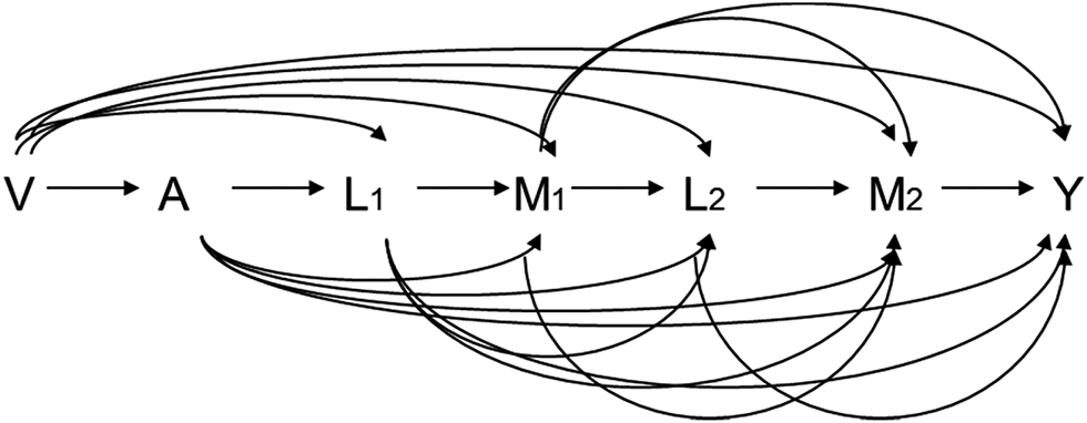
Causal diagrams for a setting with two mediators and time-varying mediator-outcome confounders affected by exposure.
Definitions of total effect (TE), control direct effect (CDE), natural direct effect (NDE), natural indirect effect (NDE), and the randomly interventional analogues of these effects
Let A = a1 and A = a0 denote two hypothetical intervention statuses (for example, exposure and non-exposure, respectively).We use counterfactual models described above to define all effects of the exposure on the outcome by comparing two exposure levels, a1 and a0. The total effect (TE) is defined as E[Y(a1)]−E[Y(a0)]. For mediation analysis, the total effect is decomposed into direct effect and indirect effect mediated by two mediators, M1 and M2. Two strategies are available for different scientific questions of interest. The first strategy assesses direct effect and indirect effect by the controlled direct effect (CDE) and the difference of TE and CDE, respectively. CDE is defined as E[Y(a1,m1,m2)]−E[Y(a0,m1,m2)], which can be interpreted as the effect of the exposure on the outcome while two mediators, M1 and M2, are intervened as certain levels, m1 and m2, respectively. The difference between the total effect and the CDE can be used to estimate the extent to which the total effect blocked by setting the mediators to a certain level and is valuable for questions about policy making. For identifying CDE, we can use two assumptions:
(1) no unmeasured exposure-outcome confounding (mathematically expressed as Y(a,m1,m2) ⊥ A|V)
(Assumption 1)
and (2) no unmeasured mediator-outcome confounding (mathematically expressed as Y(a,m1,m2)⊥M1|V, A, L1 and Y(a,m1,m2)⊥M2|V, A, L1, M1, L2)
(Assumption 2).
Under the above assumptions, CDE can be identified as
where
Q(a,m1,m2) is the g-formula proposed by Robins [26] while A, M1, and M2 are intervened as a, m1, and m2. For any random variable W, let w denote W = w in all probability function. For example,
For questions about investigation of causal mechanism, one often instead divides the TE into a natural direct effect (NDE) and a natural indirect effect (NIE), which are defined as follows [5, 12, 13]:
where Φ(a, a’), the standard mediation parameter, is defined as E[Y(a,M1(a’),M2(a’))]. NDE expresses the change of outcome given the exposure is changed from a0 to a1, but the mediators are kept at the level they would be if the exposure is set to a0. In contrast, NIE expresses the change of outcome given the exposure is set to a1 but the mediator is changed from the level it would be if exposure is set to a0 to the level it would be if exposure is set to a1. To identify the standard mediation parameter (as well as NDE and NIE) non-parametrically by empirical data, the following four assumptions suffice [12]:
(1) Assumption 1 above
(2) no unmeasured mediator-outcome confounding (mathematically expressed as Y(a,m1,m2)⊥(M1, M2)|V, A, L1)
(Assumption 2-1),
(3) no unmeasured exposure-mediator confounding (mathematically expressed as A⊥(M1(a), M2(a))|V)
(Assumption 3),
and
(4) no mediator-outcome confounders are affected by exposure (mathematically expressed by Y(a,m1,m2)⊥(M1(a), M2(a))|V)
(Assumption 4).
Although Assumption 2 and Assumption 2-1 are both interpreted as “no unmeasured mediator-outcome confounding”, the former is weaker than the latter. For example, Assumption 2-1 is violated under the presence of a M2-Y confounder affected by M1. However, Assumption 2 still holds if this confounder can be measured accurately.
Under four assumptions, Φ(a, a’), NDE, and NIE can be non-parametrically identified as Q(a, a’), Q(a1, a0)−Q(a0, a0), and Q(a1, a1)−Q(a1, a0), respectively, where Q (a,a’) =
For Assumption 4 to hold, L1 and L2 should not be present, i. e. there should be no mediator-outcome confounders affected by the exposure [13, 27], as shown in Figure 2. This strong assumption can be violated even if the two mediators occurred soon after the exposure. Therefore, alternative definitions for NDE and NIE, i. e. randomly interventional analogues of natural direct effect (rNDE) and of natural indirect effects (rNIE), have been proposed [9, 19] for settings with time-varying confounders [21, 22, 23, 24, 28]. rNDE and rNIE are defined as follows:
where the rΦ(a, a’), the randomly interventional analogue of Φ(a, a’), is defined as E[Y(a,G12(a’))], which replaces (M1(a’), M2(a’)) in Φ(a, a’) by G12(a’). The rNDE expresses the change of outcome given the exposure changes from a0 to a1 but mediators are set to the value randomly drawn from a distribution of population with exposure is set to a0. The rNIE expresses the change of outcome given the exposure is set to a1, but the mediator changes from the value randomly drawn from the distribution in the population if the exposure were set to a0 to the value randomly drawn from the distribution in the population if exposure were set to a1. The sum of rNDE and rNIE are called randomly interventional analogue of total effect (rTE).
In order to identify rΦ (as well as rNDE and rNIE), only three no unmeasured confounding assumptions (i. e., Assumption 1, Assumption 2-1, and Assumption 3) are required while Assumption 4 is no longer necessary. Since for multiple mediators, we cannot ensure all mediators occur immediately after the exposure and so the mediator-outcome confounders are thus perhaps more likely to be affected by exposure and Assumption 4 is more likely to be violated. In the next section, we will extend the approach of randomly interventional analogue to define path-specific effects in setting with multiple mediators.
Definition and identification of randomly interventional analogues of path-specific effects
In this section, we focus on the simplest case, i. e. the setting with two mediators. The notation was introduced in previous section and the causal relationship among all covariates is shown in Figure 1. When there are two mediators, the number of all possible mediator combinations is four. Therefore, TE can be divided into four path-specific effects (PSEs): (1) the path not mediated by M1 or M2 (
Four standard PSEs are defined as follows [13, 16, 17, 28]:
where Φ(a, a’, a’’, a’’’) is defined as E[Y(a,M1(a’),M2(a’’,M1(a’’’)))]. It is worth noting that the
Using a similar approach to rNDE and rNIE, we define randomly interventional analogues of PSEs (rPSEs): (1)
where rΦ(a, a’, a’’, a’’’) is defined as E[Y(a,G1(a’),G2(a’’,G1(a’’’)))], which is the randomly interventional analogue of Φ(a, a’, a’’, a’’’). The rTE can be decomposed to four rPSEs, i. e.
Before interpreting all rPSEs and rTE, we first define five populations with hypothetical intervention on exposure (and the first mediator). Let population 1 and population 0 denote the populations with exposure set to a1 and a0, respectively. Let population 1-1 and population 1-0 denote the populations with exposure set to a1 and first mediator set to a value randomly drawn from the distribution from population 1 and population 0, respectively. Similarly, population 0-0 denotes the population with exposure set to a0 and first mediator set to a value randomly drawn from the distribution of population 0. Then we can interpret rTE and four rPSEs based on the five populations. rTE expresses the change of outcome given the exposure changes from level a0 to a1, the first mediator M1 changes from a value randomly drawn from the distribution of population 0 to a value randomly drawn from the distribution of population 1, and M2 changes from a value randomly drawn from the distribution of population 0-0 to a value randomly drawn from the distribution of population 1-1.; rTE captures all paths from A to Y.
For identifying rΦ (as well as all rPSEs), it suffices to make following four no unmeasured confounding assumptions:
(1) Assumption 1,
(2) Assumption 2,
(3) no unmeasured exposure-mediator confounding (mathematically expressed as A⊥(M1(a), M2(a,m1)) |V)
(Assumption 3-1),
and (4) no unmeasured mediator-mediator confounding (mathematically expressed as M2(a,m1)⊥M1 |V, A, L1)
(Assumption 5).
Under the four assumptions, rΦ(a, a’, a’’, a’’’) can be non-parametrically identified as the following equations:
The detail proof is provided in Appendix 1 [Online], proof A and B.
All types of rPSEs and rTE can be expressed in terms of Q as follows.
The definitions and identification of rPSEs in settings with three mediators are provided in Appendix 2 [Online].
We then discuss about the relation of our method to causal mediation analysis. Consider a setting with only one mediator, i. e. the L2 and M2 are empty, and the rΦ(a, a’, a’’, a’’’) reduces to
which is the identification of E[Y(a,G(a’))] [28]. When the time-varying confounders are not affected by exposure, i. e. all L1, L2, and M2 are all empty, rΦ(a, a’, a’’, a’’’) reduces to
A regression based approach and illustration
In this section, we propose a regression based approach. The SAS code estimates effects conditional on the covariates. Marginal effects for these models can be obtained by evaluating the effects at the average value of the covariates. We also assume no time-varying confounder affected by exposure and no mediator-mediator interaction. Below we consider a single confounder V = C but we also discuss later the analogous results for multiple confounders in V.
Consider settings with binary exposure (A = a1 or A = a0), continuous mediators and outcome, and no time-varying confounder affected by exposure (Figure 2). In addition, we also assume linear regression model allowing for exposure-mediator interactions for all continuous covariates as below:
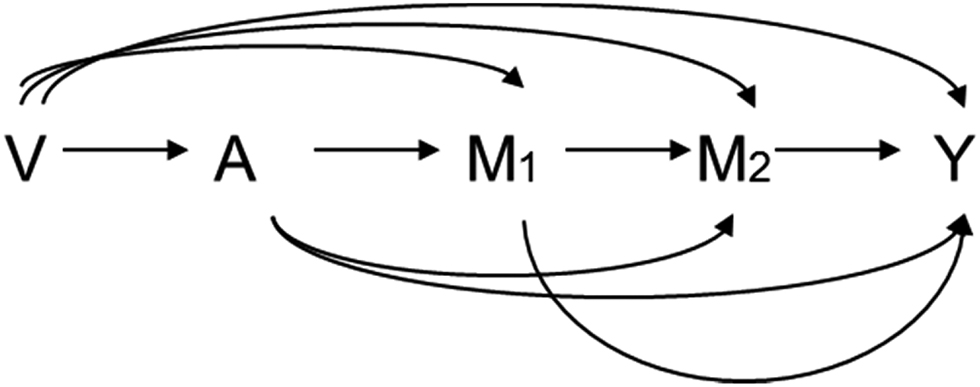
Causal diagrams for a setting with two mediators but no time-varying mediator-outcome confounders.
.
According to the formula, we can derive the following expressions for four rPSEs:
The proofs are given in Appendix 3 [Online]. Several comments merit attention. First, we include only exposure-mediator interaction here. Similar formulas can be derived allowing for mediator-mediator interaction and even three-way interaction (interaction term among A, M1, and M2). In Appendix 3 [Online], we also show the formula including mediator-mediator interaction. Second, we propose a SAS macro for applying this formula to data in Appendix 4 [Online]. The standard error is estimated by delta method. Third, when the baseline confounders are more than one, ie when c = (c1, c2, …, cp)T, we just need to replace the θc, βc, and γc by θcT = θc1, θc2, …, θcp), βcT = (βc1, βc2, …, βcp), and γcT = (γc1, γc2, …, γcp), respectively. Finally, under the above setting as well as no exposure-mediator interaction,
Illustration
We illustrate the regression based method described above by investigating the causal mechanisms of smoking behavior on systolic blood pressure (SBP) mediated by cholesterol level and body weight. Beginning in 1948 in Framingham, Massachusetts, the original Framingham cohort consisted of 5,209 participants aged from 30 to 62 years without cardiovascular disease (CVD) history at baseline. All the participants underwent examinations at the beginning of the study and routinely every two years after that. During each exam, potential CVD risk factors were collected, including socio-demographic data, lifestyle characteristics, detailed medical history, physical examination data, and blood samples. Further details on the design of FHS are described elsewhere [26], 37]. Four exclusion criteria are listed below: (1) death or loss to follow up during the period before exam 7 (the end of follow-up); (2) no record at baseline on weight, height, smoking status, former smoking history, SBP, or total cholesterol; (3) diagnosis of diabetes, cancer, or CVD at baseline; and (4) value for smoking status or BMI missing more than once. In addition, we also eliminate those who quit smoke in order to focus on the current smoker versus non-smoker comparison. After these exclusions, 2,993 participants are eligible for analysis. The analysis is intended only as an illustration of the estimation approach. SBP (mm-Hg) at exam 7 is the outcome Y and smoking amount is exposure of interest (comparing smoking for 30 cigarettes per day vs. nonsmoking). The cholesterol level (mg/dL) at exam 4 and BMI (kg/m2) at exam 6 are two mediators M1 and M2. We include gender, age (years), and baseline smoking status (smoker vs. non-smoker) as our baseline confounders. A linear regression model is fit for SBP on the cholesterol, BMI, smoking, the interaction between smoking and cholesterol level, the interaction between smoking and BMI, and the baseline covariates (gender and age). A linear regression model for BMI is fit on the smoking, cholesterol level, their interaction, and baseline covariates. A linear regression model for cholesterol level is fit on the smoking and baseline covariates. Confidence intervals are obtained using the delta method. The SAS code in the context of the rPSE decomposition is provided in the Appendix 4 [Online]. We use this decomposition and these methods so that we can separate the effect of smoking on SBP mediated directly through cholesterol to SBP versus that which changes BMI through changing cholesterol.
Results are summarized in Table 1. The SBP increases by 1.956 mm-Hg (95 % Confidence Interval [CI] = −0.6758 to 4.5879) when smoking status changed from nonsmoking to smoking 30 cigarettes per day while cholesterol level and BMI were both stochastically set to the distribution among nonsmokers; this measurement represents the effect of smoking on SBP not through cholesterol level or BMI. The SBP increases by 1.0348 mm-Hg (95 % CI = 0.4009 to 1.6687) when cholesterol level changed from being stochastically setting to the distribution of non-smokers to the distribution of smokers, while smoking amount was set to 30 cigarettes per day and BMI to the distribution of non-smokers; this measurement represents the effect of smoking on SBP through cholesterol level only. The SBP decreases by 0.1655 mm-Hg (−0.4980 to 0.8291) when BMI changes from being setting to the distribution of non-smokers to the distribution of the smokers, of which the cholesterol level was stochastically set to the distribution of non-smokers, while smoking status was set to smoking and cholesterol level was stochastically set by the distribution of smokers; this measurement represents the effect of smoking on SBP through BMI only. The change of SBP is 0.2009 mm-Hg (0.0369 to 0.3650) when BMI changed from being set to the distribution of the smokers, for which the cholesterol level was stochastically set to the distribution of non-smokers, to the distribution of smokers, while smoking amount was set to 30 cigarettes per day and cholesterol level was stochastically set to the distribution of smokers; this measurement represents the effect of smoking on SBP through cholesterol level then through BMI.
Of these 4 rPSEs, the direct effect and effect mediated by cholesterol level only are dominant highlighting the important role of cholesterol in this context. The effect mediated by BMI is non-significant but has different direction from total effect, perhaps indicating the possibility that the adverse effect of smoking on increasing blood pressure is partially concealed by body weight loss. However, this path is balanced by another path via cholesterol level and then BMI. Our results provide evidence that the cholesterol level might play an important role in the mechanism of smoking on SBP.
Proportions of the effect of smoking on systolic blood pressure mediated by cholesterol and/or body mass index.
| Effects | (95 % CI) | p-value | Proportion attributable | (95 % CI) | p-value | |
|---|---|---|---|---|---|---|
| 1.9560 | (−0.6758, 4.5879) | 0.1452 | 0.6464 | (0.2704, 1.0223) | 0.0008 | |
| 1.0348 | (0.4009, 1.6687) | 0.0014 | 0.3419 | (0.0109, 0.6730) | 0.0429 | |
| −0.1655 | (−0.8291, 0.4980) | 0.6248 | −0.0547 | (−0.2893, 0.1799) | 0.6476 | |
| 0.2009 | (0.0369, 0.3650) | 0.0164 | 0.0664 | (−0.0152, 0.1480) | 0.1108 | |
| Effect via M1 (with/without M2) | 1.2357 | (0.5488, 1.9226) | 0.0004 | 0.4083 | (0.0173, 0.7994) | 0.0407 |
| Effect via M2 (with/without M1) | 0.0354 | (−0.6426, 0.7134) | 0.9184 | 0.0117 | (−0.2105, 0.2339) | 0.9178 |
| Effect via M1 or M2 | 1.0702 | (0.1195, 2.0209) | 0.0274 | 0.3536 | (−0.0223, 0.7296) | 0.0652 |
| rTE | 3.0262 | (0.2679, 5.7846) | 0.0315 | 1 |
Discussion
To understand the mechanisms with multiple mediators, it is necessary to investigate all PSEs. When the mediators affect to each other, the analysis will become complicated since one path might be shared by several PSEs. In the setting with two mediators, the path from A to M1 belongs to both
Rather than the standard definitions based on cross-world counterfactual outcomes, our method used definitions of randomly interventional analogues, which is not exactly how the mechanisms perform in nature. It corresponds to intervening on the mediator to equalize their distributions across exposure levels. The sum of all rPSEs is rTE, rather than total effect of exposure on outcome. It is also worth to note that these effects can be examined in principle in randomized controlled trial, while PSEs cannot since PSEs are defined using cross-world counterfactual outcomes [27].
Although rPSEs as well as rTE are not identical to the traditional definitions, they might be the best we can do for mechanism investigation as only fairly wide bounds of the traditional path-specific effect can be identified even under strong assumptions. As analogues of PSEs, the rPSEs still capture pathways; for example,
Besides the deviation from traditional definition, two limitations concerning our method merit discussion. First, assumptions of no unmeasured confounding are required for accurate rPSE estimates. To ensure these assumptions held, researchers should collect all potential confounders as comprehensively as possible. When collection of all covariates is impossible, sensitivity analysis techniques could be developed to assess the extent of bias due to assumption violation. In addition, our SAS code only allows linear regression model with exposure-mediator interaction. Methods allowing binary or time to event outcome could be developed but are not yet available. For applying this method more broadly, more methods and corresponding software could be developed in the future.
In conclusion, our study provides a framework to decompose rTE into several rPSEs mediated by all possible combinations of mediators, extending the standard analysis method to settings with interaction, non-linearity, and time-varying confounders affected by exposure. Our method contributes to the investigation of complicated causal mechanisms in settings with multiple mediators.
Declarations of competing interest
None.
Reference
1. Robins JM, Greenland S. Identifiability and exchangeability for direct and indirect effects. Epidemiology 1992;3(2):143–155.10.1097/00001648-199203000-00013Search in Google Scholar PubMed
2. Pearl J. (2001). Direct and indirect effects."Proceedings of the seventeenth conference on uncertainty in artificial intelligence", edited by Breese J, Koller D. San Francisco, CA, USA: Morgan Kaufmann Publishers Inc. 411-420Search in Google Scholar
3. VanderWeele T, Vansteelandt S. Conceptual issues concerning mediation, interventions and composition. Stat Interface 2009;2:457–468.10.4310/SII.2009.v2.n4.a7Search in Google Scholar
4. van der Laan MJ, Petersen ML. Direct effect models. Int J Biostat 2008;4(1):Article 23.10.2202/1557-4679.1064Search in Google Scholar PubMed
5. VanderWeele TJ. Marginal structural models for the estimation of direct and indirect effects. Epidemiology 2009;20(1):18–26.10.1097/EDE.0b013e31818f69ceSearch in Google Scholar PubMed
6. Imai K, Keele L, Tingley D. A general approach to causal mediation analysis. Psychol Methods 2010;15(4):309.10.1037/a0020761Search in Google Scholar PubMed
7. VanderWeele TJ. Bias formulas for sensitivity analysis for direct and indirect effects. Epidemiology (Cambridge, Mass.) 2010;21(4):540.10.1097/EDE.0b013e3181df191cSearch in Google Scholar PubMed PubMed Central
8. VanderWeele TJ, Vansteelandt S. Odds ratios for mediation analysis for a dichotomous outcome. Am J Epidemiol 2010;172(12):1339–1348.10.1093/aje/kwq332Search in Google Scholar PubMed PubMed Central
9. Didelez V, Dawid P, Geneletti S. Direct and indirect effects of sequential treatments 2012. arXiv preprint arXiv:1206.6840.Search in Google Scholar
10. Tchetgen EJT, Shpitser I. Semiparametric theory for causal mediation analysis: efficiency bounds, multiple robustness and sensitivity analysis. Ann Stat 2012;40(3):1816–1845.10.1214/12-AOS990Search in Google Scholar PubMed PubMed Central
11. Valeri L, VanderWeele TJ. Mediation analysis allowing for exposure–mediator interactions and causal interpretation: theoretical assumptions and implementation with SAS and SPSS macros. Psychol Methods 2013;18(2):137.10.1037/a0031034Search in Google Scholar PubMed PubMed Central
12. VanderWeele TJ, Vansteelandt S. Mediation analysis with multiple mediators. Epidemiol Method 2014;2(1):95–115.10.1515/em-2012-0010Search in Google Scholar PubMed PubMed Central
13. Avin C, Shpitser I, Pearl J. Identifiability of path-specific effects 2005. Department of Statistics, UCLA.Search in Google Scholar
14. Shpitser I. Counterfactual graphical models for longitudinal mediation analysis with unobserved confounding. Cognit Sci 2013;37(6):1011–1035.10.1111/cogs.12058Search in Google Scholar
15. Shpitser I, Tchetgen ET. Causal inference with a graphical hierarchy of interventions 2014. arXiv preprint arXiv:1411.2127.Search in Google Scholar
16. Albert JM, Nelson S. Generalized causal mediation analysis. Biometrics 2011;67(3):1028–1038.10.1111/j.1541-0420.2010.01547.xSearch in Google Scholar
17. Daniel R, De Stavola B, Cousens S, Vansteelandt S. Causal mediation analysis with multiple mediators. Biometrics 2015;71(1):1–14.10.1111/biom.12248Search in Google Scholar
18. Taguri M, Featherstone J, Cheng J. Causal mediation analysis with multiple causally non-ordered mediators. Stat Methods Med Res 2015. 0962280215615899.10.1177/0962280215615899Search in Google Scholar
19. Geneletti S. Identifying direct and indirect effects in a non‐counterfactual framework. J R Stat Soc Ser B (Stat Method) 2007;69(2):199–215.10.1111/j.1467-9868.2007.00584.xSearch in Google Scholar
20. VanderWeele TJ, Robinson WR. On causal interpretation of race in regressions adjusting for confounding and mediating variables. Epidemiology (Cambridge, Mass.) 2014;25(4):473.10.1097/EDE.0000000000000105Search in Google Scholar
21. Zheng W, van der Laan MJ. Causal mediation in a survival setting with time-dependent mediators. U.C. Berkeley Division of Biostatistics Working Paper Series 2012;Working Paper:295.Search in Google Scholar
22. VanderWeele TJ, Tchetgen Tchetgen E. Mediation analysis with time-varying exposures and mediators. J R Stat Soc Ser B (Stat Method) 2016. DOI: 10.1111/rssb.12194. (accepted)Search in Google Scholar
23. Lin S-H, Young J, Tchetgen Tchetgen E, VanderWeele TJ. Parametric mediational g-formula approach to mediation analysis with time-varying exposures, mediators and confounders: an application to smoking, weight, and blood pressure. Epidemiology 2016. (accepted).10.1097/EDE.0000000000000609Search in Google Scholar
24. Lin S-H, Tchetgen Tchetgen E, Young J, Logan R, VanderWeele TJ. Mediation analysis with survival outcome and time-varying exposures, mediators, and confounders: a case study of the Framingham heart study. 2015. submitting.Search in Google Scholar
25. Pearl J. Causal inference in statistics: an overview. Stat Surv 2009;3:96–146.10.1214/09-SS057Search in Google Scholar
26. Robins J. A new approach to causal inference in mortality studies with a sustained exposure period – application to control of the healthy worker survivor effect. Math Modell 1986;7(9):1393–1512.10.1016/0270-0255(86)90088-6Search in Google Scholar
27. VanderWeele T. Explanation in causal inference: methods for mediation and interaction. Oxford: Oxford University Press, 2015.10.1093/ije/dyw277Search in Google Scholar
28. VanderWeele TJ, Vansteelandt S, Robins JM. Effect decomposition in the presence of an exposure-induced mediator-outcome confounder. Epidemiology 2014;25(2):300–306.10.1097/EDE.0000000000000034Search in Google Scholar PubMed PubMed Central
29. MacKinnon DP. Introduction to statistical mediation analysis. Abingdon: Routledge, 2008.Search in Google Scholar
Supplemental Material
The online version of this article (DOI:https://doi.org/10.1515/jci-2015-0027) offers supplementary material, available to authorized users.
© 2017 Walter de Gruyter GmbH, Berlin/Boston
This article is distributed under the terms of the Creative Commons Attribution Non-Commercial License, which permits unrestricted non-commercial use, distribution, and reproduction in any medium, provided the original work is properly cited.
Articles in the same Issue
- Research Articles
- Design and Analysis of Experiments in Networks: Reducing Bias from Interference
- Interventional Approach for Path-Specific Effects
- Entropy Balancing is Doubly Robust
- Semi-Parametric Estimation and Inference for the Mean Outcome of the Single Time-Point Intervention in a Causally Connected Population
- Identification of the Joint Effect of a Dynamic Treatment Intervention and a Stochastic Monitoring Intervention Under the No Direct Effect Assumption
- Causal, Casual and Curious
- A Linear “Microscope” for Interventions and Counterfactuals