Interaction between Interfacial Collinear Griffith Cracks in Composite Media under Thermal Loading
-
P.K. Mishra


Abstract
This article deals with the interactions between a central crack and a pair of outer cracks situated at the interface of orthotropic elastic half planes under thermo-mechanical loading. The mixed boundary value problem has been reduced to a pair of singular integral equations which has been solved numerically using Jacobi polynomial method. The interaction effects have been obtained in terms of stress magnification factors depending on the crack spacing and crack length. The phenomena of crack shielding and crack amplification have been depicted through graphs for different particular cases.
1 Introduction
It looks that microscopic flows do not lead to safe structure to fail. Sometimes, it becomes very expensive to replace the component of engineering structures. In fact, on one hand, due to increasing demands for energy and material conservations, the safety margins assigned to structures have to be smaller. On the other hand, the detection of a flaw in a structure does not automatically mean that it is not safe to use anymore. This is particularly relevant in the case of expensive materials or components of structures whose usage it would be inconvenient to interrupt. In this setting fracture, mechanics plays a key role during the analysis of materials which exhibits cracks and also to predict whether and in which manner failure may occur.
A property of a structure relating to its ability to sustain defects until repair is called damage tolerance. During design of engineering structures, the damage tolerance is always taken in account as it is assumed that flaws can exist in any structure and such flaws propagate with usage. In aerospace engineering structures, this approach is necessary to avoid the extension of cracks. In fracture mechanics, crack growth is exponential in nature, that is, the crack growth rate is a function of an exponent of crack size according to the Paris law. The exponential crack growths led to the development of non-destructive testing methods through which the structural engineers may inspect invisible cracks occur in structures which grow slowly. So amounts of maintenance checks are reduced by nondestructive inspections. Crack propagation and arrest have become important topics in a structure containing isolated region of an unstable crack growth. So emergence of an unstable crack from bad region can still be arrested using the surrounding of good materials, provided good materials have sufficiently high fracture toughness i.e., materials have large resistance to protect the structure from crack propagation. This clearly exhibits the importance of studying propagation of cracks occur in structures and the arrest of crack propagation for the safety of the structure. The physical quantities such as stress intensity factor, crack energy, stress magnification factor (SMF) play important roles during the study of crack arrest [1–8].
Problems consist of heat and deformation that has attracted much interest to the scientists and engineers for last couple of decades. The thermal stress concentration near the crack tips has become an interesting topic of research nowadays. In the formation of structural members of airplanes, motor vehicles and high speed trains, composite materials are used widely due to their light weight and strong nature. When a cracked structural member is subject to different temperature fields, then the evaluation of stress intensity factors becomes essential due to disturbance in heat flux. The study of thermal stress around the cracked surface becomes important for the prediction of stability and service life of cracked engineering materials and structures. In linear elastic fracture mechanics, the study of geometry of collinear cracks has practical importance as pre-existing cracks lead to fracture due to interaction of cracks which forms a major crack in a medium. In 2002, Noda and Wang [9] have studied the interaction between collinear cracks situated in an inhomogeneous medium under transient loading. During thermo elastic analysis of a cracked solid, a considerable effort has been given by the researchers based on the theory of the thermo-elasticity. In 1962, Sih [10] observed the singular character of thermal stress near a crack in an infinite plate when heat flows perpendicular to the crack. A solution of a thermo-elastic crack problem had been given by Atkinson and Clement [11] in an anisotropic medium with single crack. Applying the method given by Muskhelishvili [12], Clement [13] solved the thermo-elastic crack problem bonded between dissimilar anisotropic materials. He assumed that the heat flows through the two surfaces of a crack equally but opposite in direction. In 1977, Sekine [14] calculated the thermal stresses near the crack tips of an isolated line crack in a semi-infinite medium subjected to uniform heat flow. In 1979, same author studied thermo-elastic interaction between two cracks [15]. In 1991, Itou [16] has calculated the thermal stresses around an isolated crack in an infinite elastic strip in which the surfaces of the strip are maintained at different temperature. In 1993, Itou and Rengen [17] studied the thermal stresses around two parallel cracks situated at the interface positions of two bonded dissimilar elastic half planes. In 1995, Itou and Rengen [18] have solved a problem of two collinear cracks in an adhesive layer sandwiched between two dissimilar elastic half planes. In 2001, thermal stresses in an infinite orthotropic plate around two parallel cracks under uniform heat flow were evaluated by Itou [19]. In 2007, Zhou et al. [20] have investigated transient two-dimensional thermal crack problem in a functionally graded orthotropic strip using Laplace and Fourier transform techniques. In 2007, Baksi et al. [21] have determined the thermal stresses and displacement fields in an orthotropic plane containing a pair of equal collinear Griffith cracks using integral transform technique based on displacement potential functions under steady-state temperature field. In 2013, Zhong et al. [22] have investigated the thermal stress around two collinear Griffith cracks in an orthotropic solid subjected to thermo-mechanical loading using Fourier transform technique. Recently, Itou [23] has calculated the thermal stress in an infinite orthotropic plane around two upper collinear cracks placed parallel to a lower crack. Problem related to thermal stress can also be found in the research articles [24–29]. But to the best of authors’ knowledge, the problem related to interaction between interfacial cracks under thermo-mechanical loading are not yet been done by any researcher.
The main goal of this article is to analyze the interaction among three collinear Griffith cracks situated at the interface of two orthotropic thermo-elastic half planes under uniform heat flux. To study the effect of temperature on displacements and stresses, an integral technique has been applied. The problem is reduced to a dual form of the integral equations, which is solved numerically using Jacobi polynomials. The expressions of SIFs at the tips of the cracks are found analytically. The graphical presentations of the effect of outer cracks on the propagation of central crack and also the propagation tendency of outer crack due to the presence of central one for different particular cases are the key feature of this article.
2 Problem Formulation
Consider two bonded homogeneous orthotropic elastic half planes y≥0 and y≤0 containing three collinear Griffith cracks at the interface of y=0 when Cartesian co-ordinate axes coincide with the axes of symmetry of the elastic material. When thermal conditions are applied to the surface of an arbitrary two-dimensional orthotropic half planes, then temperature field only depends on in-plane co-ordinates under steady-state condition. The temperature distribution functions T(i) (x,y) are assumed to satisfy the following heat conduction equation in the orthotropic media as
where
The general solution of T(j) (x,y) is (c.f., Akoz and Tauchert [30])
where
Here, we have assumed that
and hence the Fourier integral form of temperature distribution may be written as
From (2) and (4), we get
From (2) and (5), the temperature distribution T(i)(x,y) can be expressed as
Consider
where h(x) is the prescribed temperature distribution, which becomes line source along y-axis, and δ(x) is Dirac delta function. Therefore, resultant temperature distribution is reduced to
The relations between plane stress induced by the distributions of temperature and displacement components u(i) and v(i) are given by
The elastic constants are given by
The displacement equations of equilibrium are given by
in which u(i)=u(i)(x, y), v(i)=v(i)(x, y) are the displacement components along x- and y-directions. It is assumed that at the interface y=0, the central crack defined by |x|<a and the outer defined by b<|x|<1 are opened by internal normal and shearing tractions p1(x) and p2(x), respectively (Figure 1). The boundary conditions on y=0 are given by

Geometry of the problem.
In Figure 1, the inclined arrows represent the regions for the semi-infinite half planes, the vertical arrows denote the direction of the applied normal stress and the horizontal arrows denote the direction of shearing stress for our considered mixed mode type problem.
3 Solution of the Problem
During solution of the problem, we first introduce displacement potentials ψ(i)(x, y) and
Potential functions for the half planes are given by
The displacement components u(i) and v(i) may be written as
The corresponding thermal stresses are
The displacement equations (12) and (13) are satisfied by (20) for nontrivial
Here, potential functions
where
Boundary conditions (16) and (17) with the help of above-mentioned equations give rise to
Now setting
where
and after lengthy process of mathematical manipulations, boundary conditions (14) and (15) finally lead to the following singular integral equations
where
Equations (31) and (32) are reduced to the following singular integral equations for the determination of unknown functions fi(x) satisfying the conditions
where
The solution of above integral equations (34) may be assumed as
where
and
with ckn are unknown constants. Now using (33), we get
which implies ck0=0, k=1, 2.
From (31) and (32), we get
Multiplying the above-mentioned equation by
where
with k=1, 2, j=0, 1.
and the principal value of
Finally, the stress intensity factors at the crack tips at x=a, x=b and x=1 are calculated as
Now SMFs are defined by
4 Numerical Results and Discussion
In this section, the numerical computations have been done to find physical quantities viz., stress intensity factors and stress magnification factors for three collinear cracks situated at the interface of two orthotropic materials as α-Uranium and Epoxy Boron. The elastic constants of the orthotropic material α-Uranium have been taken as C11=21.47×10⁶ psi (148.03 GPa), C12=4.65×10⁶ psi (32.06 GPa), C22=19.36×10⁶ psi (133.48 GPa),
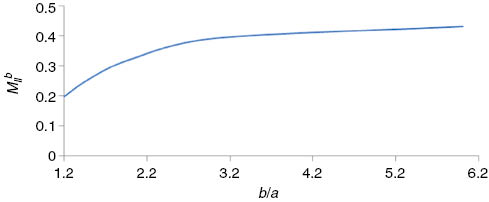
C66=7.43×10⁶ psi (51.22 GPa) (Mukherjee and Das [5]). The elastic constants of the other considered orthotropic material Boron-Epoxy have been taken as C11=30.3×10⁶ psi (208.91 GPa), C12=3.78×10⁶ psi (26.06 GPa), C22=4.04×10⁶ psi (27.85 GPa), C66=1.13×10⁶ psi (7.79 GPa) (Sih and Chen [32]). During computations, the loadings are considered to be p1(x)=p, p2(x)=0. The dimensionless stress magnification factors for both the Mode-I and Mode-II types at the tip of the central crack x=a are described through Figures 2 and 3, respectively, for different values of dimensionless quantity b/a keeping a=0.5 and varying b=0.6(0.1) 0.9. Again keeping the outer crack length fixed b=0.6 and varying a=0.1(0.1) 0.5, the stress magnification factors at the outer crack tips x=b and x=1 are depicted through Figures 4–7, respectively, for various values of b/a for Mode-I and Mode-II types.

Plot of

Plot of

Plot of
Plot of

Plot of

Plot of
It is seen from Figure 2 that as the length of the outer crack increases, then stress magnification factor
The variations of mode-II stress magnification factor depend on the crack separation distance and crack length. Figure 3 shows that central crack experiences shielding effect due to the presence of outer crack. This effect is maximum when outer crack size is minimum and crack separation distance between the outer crack and central crack is maximum. As the length of the outer crack decreases together with simultaneous increase in crack separation, the shielding effect increases gradually. When the outer crack size is 40% and crack separation distance is 10% of main crack size then shielding is about 45%. When the size of the outer cracks is one-twentieth and crack separation is nine-twentieth to the central crack, then shielding is about 80%.
Figure 5 reveals that outer crack experiences shielding effect due to the presence of central crack. This effect is maximum when central crack size is maximum and crack separation distance between the outer crack and central crack is minimum. As the length of the central crack decreases together with simultaneous increase in crack separation distance, the shielding effect gradually decreases. When the central crack size is 120% and crack separation distance is 25% to the outer crack size, then shielding is about 80%. When the size of the central crack is half and crack separation is five-forth to the outer crack, then shielding is about 60%.
5 Conclusion
In this article, the authors have achieved three important goals. The first one is the investigation of three collinear cracks at the interface of two orthotropic media under thermo-mechanical loading. Second one is finding the analytical form of the stress intensity factors at the vicinity of the crack tips. Third one is the graphical presentations of amplification and shielding effect through the stress magnification factors which helps to find the possibilities of arrest of central crack due to the presence of outer cracks and vice versa.
Acknowledgments
The authors of the article express their heartfelt thanks to the revered reviewers for their valuable suggestions for the improvement of the article.
References
[1] P. H. Melville, Int. J. Fract. 13, 165 (1977).10.1007/BF00042558Search in Google Scholar
[2] L. R. F. Rose, Int. J. Fract. 3, 233 (1986).10.1007/BF00018929Search in Google Scholar
[3] A. Misra and A. A. Sukere, Int. J. Fract. 52, R37 (1991).10.1007/BF00034908Search in Google Scholar
[4] A. H. Priest, Eng. Fract. Mech. 61, 231 (1998).10.1016/S0013-7944(98)00075-7Search in Google Scholar
[5] S. Mukherjee and S. Das, Int. J. Solids Struct. 44, 5437 (2007).10.1016/j.ijsolstr.2006.10.024Search in Google Scholar
[6] A. Bousquet, S. Marie, and P. Bompard, Comput. Mater. Sci. 64, 17 (2012).10.1016/j.commatsci.2012.04.026Search in Google Scholar
[7] G. T. Hahn and M. F. Kanninen (Editors), Fast Fracture and Crack extension, American Society for Testing and Materials (1976).10.1520/STP627-EBSearch in Google Scholar
[8] P. K. Mishra, S. Das, and M. Gupta, Zamm–J. Appl. Math. Mech., doi: 10.1002/zamm.201500102 (2016).10.1002/zamm.201500102Search in Google Scholar
[9] N. Noda and B. L. Wang, Acta Mech. 153, 1 (2002).10.1007/BF01177046Search in Google Scholar
[10] G. C. Sih, ASME J. Appl. Mech. 29, 587 (1962).10.1115/1.3640612Search in Google Scholar
[11] C. Atkinson and D. L. Clement, Int. J. Solids Struct. 13, 855 (1977).10.1016/0020-7683(77)90071-3Search in Google Scholar
[12] N. I. Muskhelishvili, Some Basic Problems of the Mathematical Theory of Elasticity, P. Noordhoff, Groningen 1953.Search in Google Scholar
[13] D. L. Clement, Int. J. Solids Struct. 19, 121 (1983).10.1016/0020-7683(83)90003-3Search in Google Scholar
[14] H. Sekine, Eng. Fract. Mech. 9, 499 (1977).10.1016/0013-7944(77)90041-8Search in Google Scholar
[15] H. Sekine, Trans. Japan Soc. Mech. Eng. 45, 1058 (1979).10.1299/kikaia.45.1058Search in Google Scholar
[16] S. Itou, Trans. Japan Soc. Mech. Eng. 57, 1752 (1991).10.1299/kikaia.57.1752Search in Google Scholar
[17] S. Itou and Q. Rengen, Arc. Appl. Mech. 63, 377 (1993).10.1007/BF00805738Search in Google Scholar
[18] S. Itou and Q. Rengen, J. Therm. Stresses 18, 185 (1995).10.1080/01495739508946298Search in Google Scholar
[19] S. Itou, J. Therm. Stresses 24, 677 (2001).10.1080/014957301300194832Search in Google Scholar
[20] Y. T. Zhou, X. Li, and J. Q. Qin, J. Therm. Stresses 30, 1211 (2007).10.1080/01495730701519607Search in Google Scholar
[21] A. Baksi, S. Das, and R. K. Bera, Int. J. Pure Appl. Math. 36, 365 (2007).Search in Google Scholar
[22] X. C. Zhong, B. Wua, and K. S. Zhang, Theo. Appl. Fract. Mech. 65, 61 (2013).10.1016/j.tafmec.2013.05.009Search in Google Scholar
[23] S. Itou, J. Theo. Appl. Fract. Mech. 52, 617 (2014).Search in Google Scholar
[24] B. Chen and X. Zhang, J. Northwestern Polytech. Univ. 11, 121 (1993).Search in Google Scholar
[25] S. Itou, J. Therm. Stresses 16, 373 (1993).10.1080/01495739308946236Search in Google Scholar
[26] N. Noda, R. B. Hetnarski, and Tanigawa, Thermal Stresses, Taylor & Francis, New York 2003.Search in Google Scholar
[27] R. B. Hetnarski and J. Ignaczak, The Mathematical Theory of Elasticity, CRC Press, Boca Raton 2010.Search in Google Scholar
[28] M. R. Eslami, R. B. Hetnarski, J. Ignaczak, N. Noda, N. Sumi, and Y. Tanigawa, Theory of Elasticity and Thermal Stresses – Explanations, Problems and Solutions, Springer, Dordrecht 2013.10.1007/978-94-007-6356-2Search in Google Scholar
[29] R. B. Hetnarski and M. R. Eslami, Thermal Stresses – Advanced Theory and Applications, Springer, New York 2009.Search in Google Scholar
[30] A. Y. Akoz and T. R. Tauchert, J. Appl. Mech. 39, 88 (1972).10.1115/1.3422675Search in Google Scholar
[31] B. Sharma, J. Appl. Mech. 2, 86 (1958).10.1115/1.4011693Search in Google Scholar
[32] G. C. Sih and E. P. Chen, Cracks in Composite Materials, Martinus Nijhoff Publishers, The Netherlands 1981.10.1007/978-94-009-8340-3Search in Google Scholar
©2016 by De Gruyter
Articles in the same Issue
- Frontmatter
- Mechanical and Electronic Properties of P42/mnm Silicon Carbides
- Quantum Ion-Acoustic Oscillations in Single-Walled Carbon Nanotubes
- Boundary Conditions for the DKP Particle in the One-Dimensional Box
- Impact of Velocity Slip and Temperature Jump of Nanofluid in the Flow over a Stretching Sheet with Variable Thickness
- A Darboux Transformation for Ito Equation
- High-Pressure Elastic Constant of Some Materials of Earth’s Mantle
- Conservation laws and Exact Solutions of Phi-Four (Phi-4) Equation via the (G′/G, 1/G)-Expansion Method
- Noether Symmetry Analysis of the Dynamic Euler-Bernoulli Beam Equation
- Properties of Bessel Function Solution to Kepler’s Equation with Application to Opposition and Conjunction of Earth–Mars
- Interaction between Interfacial Collinear Griffith Cracks in Composite Media under Thermal Loading
- A Procedure to Construct Conservation Laws of Nonlinear Evolution Equations