A collection of machine learning assisted distributed fiber optic sensors for infrastructure monitoring
-
Christos Karapanagiotis
Christos Karapanagiotis received the Diploma in Physics from the Aristotle University of Thessaloniki, Greece, and his M.Sc. degree in Optics and Photonics from the Karlsruhe Institute of Technology (KIT), Germany, in 2018. Currently, he conducts research at the Federal Institute for Materials Research and Testing (BAM), Germany, and his research interests include distributed fiber optic sensors and machine learning in non-destructive testing (NDT) applications.
 ,
Konstantin Hicke
,
Konstantin Hicke
Konstantin Hicke received his Diploma in physics from TU Berlin in 2009 and his PhD in physics from the University of the Balearic Islands (UIB), Palma, in 2014. His PhD thesis focused on nonlinear dynamics, chaos and synchronization effects in coupled semiconductor lasers and their usage for brain-inspired photonic data processing. He has been with BAM researching and developing fiber optic sensors since 2016. His current research interests include: distributed fiber optic sensing, distributed acoustic sensing (DAS), infrastructure and condition monitoring, large-scale hazard and threat detection using fiber optic sensing, and Machine Learning assisted fiber optic sensing.
 and
Katerina Krebber
and
Katerina Krebber
Katerina Krebber studied physics and received the PhD degree in electrical engineering. She has more than 20 years experiences with the development of fibre optic sensors including distributed fibre optic sensors, FBG sensors, fibre optic radiation sensors and polymer optical fibre sensors. Since 2004 she has been with BAM. At BAM she is head of the Division Fibre Optic Sensors (BAM - Division 8.6 - Fibre Optic Sensors) and leader of a number of R&D projects. She is an author and a co-author of more than 200 scientific publications including 45 peer reviewed papers and book chapters, 120 proceedings papers, 25 invited and keynote lectures and patents. A comprehensive bibliography can be obtained from the BAM Publication Server PUBLICA.

Abstract
In this paper, we present a collection of machine learning assisted distributed fiber optic sensors (DFOS) for applications in the field of infrastructure monitoring. We employ advanced signal processing based on artificial neural networks (ANNs) to enhance the performance of the dynamic DFOS for strain and vibration sensing. Specifically, ANNs in comparison to conventional and computationally expensive correlation and linearization algorithms, deliver lower strain errors and speed up the signal processing allowing real time strain monitoring. Furthermore, convolutional neural networks (CNNs) are used to denoise the dynamic DFOS signal and enable useable sensing lengths of up to 100 km. Applications of the machine learning assisted dynamic DFOS in road traffic and railway infrastructure monitoring are demonstrated. In the field of static DFOS, machine learning is applied to the well-known Brillouin optical frequency domain analysis (BOFDA) system. Specifically, CNN are shown to be very tolerant against noisy spectra and contribute towards significantly shorter measurement times. Furthermore, different machine learning algorithms (linear and polynomial regression, decision trees, ANNs) are applied to solve the well-known problem of cross-sensitivity in cases when temperature and humidity are measured simultaneously. The presented machine learning assisted DFOS can potentially contribute towards enhanced, cost effective and reliable monitoring of infrastructures.
Zusammenfassung
In diesem Beitrag stellen wir eine Sammlung von verteilten faseroptischen Sensoren (DFOS) vor, die mit Hilfe von Maschinellem Lernen arbeiten und für Anwendungen im Bereich der Infrastrukturüberwachung geeignet sind. Wir setzen hierbei fortschrittliche Signalverarbeitung auf der Grundlage Künstlicher Neuronaler Netze ein, um die Leistungsfähigkeit dynamischer DFOS für die Messung von Dehnungen und Vibrationen zu verbessern. Insbesondere Künstliche Neuronale Netze (ANNs) liefern im Vergleich zu konventionellen und rechenintensiven Korrelations- und Linearisierungsalgorithmen geringere Dehnungsfehler und beschleunigen die Signalverarbeitung, so dass eine Dehnungsüberwachung in Echtzeit möglich ist. Darüber hinaus wenden wir Convolutional Neural Networks (CNNs) an, um dynamische DFOS-Signale zu entrauschen und damit nutzbare Messlängen von bis zu 100 km zu ermöglichen. Es werden Anwendungsbeispiele dieser durch Maschinelles Lernen unterstützten dynamischen DFOS in den Bereichen des Straßenverkehrsmonitorings und der Zug- und Gleisüberwachung aufgezeigt. Im Bereich der statischen DFOS wird Maschinelles Lernen auf das Verfahren der Optischen Brillouin-Frequenzbereichsanalyse (BOFDA) angewendet. Insbesondere CNN erweisen sich hier als sehr robust gegenüber verrauschten Spektren und tragen zu deutlich kürzeren Messzeiten bei. Darüber hinaus werden verschiedene Algorithmen des maschinellen Lernens (lineare und polynome Regression, Entscheidungsbäume, ANNs) angewandt, um das bekannte Problem der Querempfindlichkeit bei DFOS in den Fällen zu lösen, in denen Temperatur und Feuchtigkeit gleichzeitig gemessen werden sollen. Die hier vorgestellten, durch Maschinelles Lernen unterstützten, DFOS können zu einer verbesserten, kostengünstigen und zuverlässigen Überwachung von Infrastrukturen beitragen.
1 Introduction
Distributed fiber optic sensors (DFOS) have already been used for a broad range of different infrastructure monitoring purposes in practice with many more being currently investigated [1]. The most common measurands are usually strain (distributed strain sensing – DSS), temperature (DTS) and acoustics/vibrations (DAS/DVS). However, a much broader range of variables can be measured directly or indirectly using DFOS, e.g., displacement [2, 3], pressure, force, relative humidity [4–9] radiation [10–12], gas concentration [13, 14] and others.
The advantages to use DFOS technology for infrastructure monitoring purposes, apart from the many different measurable variables, are manifold. The distributedness, i.e., the possibility to continuously measure without a gap over large distances (many tens of kilometers) should be considered the most important one. The distributed nature of DFOS provides one with the opportunity to collect spatial (and possibly temporal) profiles of the measurand of interest, which can, e.g., be projected onto certain geometries. The gapless profiles can greatly simplify data evaluation and make interpolation like with conventional point sensors unnecessary. Moreover, particular signal features, anomalies or even the existence of a significant signal can be localized with great precision and accuracy over the entire sensing range. Furthermore, DFOS require mostly one, sometimes two points of access only and can fit into confined spaces easily due to their small size. They are also inherently immune to electromagnetic fields, can be employed in hazardous environments and do not require electricity or cabling where they are measuring. The fiber optic sensors themselves can be considered cost-effective (due to their possible range), robust sensing solutions that require little or no maintenance and can be embedded into infrastructure or to its surface. DFOS can be used for permanent monitoring of infrastructure or for intermittent inspection measurements. All the above make clear, that DFOS is an excellently suited technology with a proven potential for many infrastructure monitoring applications.
Distributed strain and temperature sensing based on the Brillouin effect in optical fibers have been utilized for condition monitoring of geotechnical installations, like dikes or dams [15, 16]. Pipelines have been monitored using DTS systems based on Raman or Brillouin scattering to detect leaks via the Joule–Thompson effect [17] or by employing DAS for security monitoring purposes [18] (third-party interference) or for acoustic leak detection as well [19–21]. Furthermore, extended energy infrastructure like submarine power cables [22–26] or natural gas storage cavern installations [27] are being monitored using DFOS to ascertain their condition or to detect threats to their safe operation. Moreover, the use of DAS for the monitoring of large-scale transport and traffic infrastructure like railway tracks [28–31] or roads [32, 33] to localize traffic or detect damages is being investigated as well, while DAS-based railroad monitoring is already being implemented to some degree [34]. Structural health monitoring (SHM) of civil engineering infrastructures like bridges [35, 36] or tunnels [2] is another important field of application of DFOS [37]. Finally, one field of research gaining significant interest in recent years, is using DAS for seismic measurement applications [38–43]. The use of Machine Learning for DAS data treatment and processing is particularly important in this area of research [44, 45]. Fiber optic sensors can be embedded into concrete structures (bridges), can be applied to surfaces (pipelines), can be rolled out using dedicated transducer technology like geotextiles (tunnels, dikes), can be integrated into components (power cables) or attached to parts of the installations to be monitored (caverns, tunnels). Some applications allow for the use of already laid-out fiber optic cables intended for telecom purposes (railways, roads).
All these different applications are faced with a specific set of challenges or difficult requirements attached to them, many of which can be mitigated or overcome by the use of machine learning [46, 47]. Machine learning contributed towards the development of new multiparameter fiber optic sensors alleviating the cross-sensitivity effects without increasing the cost and complexity of the system’s hardware and allowing the use of a single optical fiber [4, 48–50]. Furthermore, due to the multidimensional and complex raw data of some DFOS systems, advanced signal processing based on state-of-the-art machine learning proved advantageous over traditional methods based on correlation, linearization and least-square curve fitting algorithms [51]. Specifically, machine learning enabled real-time strain and vibration sensing replacing conventional computationally expensive algorithms, enhanced the performance increasing the measurands’ accuracy, proved more tolerant against noise allowing ultra-long sensing and uncovered more insights from the data [48, 52–56]. Machine learning has also been used to denoise the DFOS spectra outperforming conventional denoisers [57–60].
The DFOS techniques presented in this paper can be subdivided into two groups: sensing approaches with working principles based on the measurement of Rayleigh backscatter in optical fibers (“Rayleigh-based”) and those based on the Brillouin backscatter (“Brillouin-based”). Together with Raman scattering, they are the three major mechanisms used in DFOS. Rayleigh backscatter provides the strongest signal, does not require averaging, Rayleigh-based DFOS thus allows for dynamic sensing, like distributed acoustic sensing (DAS), e.g., for vibration monitoring. Brillouin-based sensing is better suited for static or quasi-static monitoring due to the low intensity of Brillouin backscatter making averaging necessary. Nonetheless, it is best suited for absolute and/or long-term monitoring applications since measurements can be referenced with offset measurements purely based on fiber material-inherent properties. Distributed temperature sensing (DTS) or distributed strain sensing (DSS) are common uses of Brillouin systems. The precision of Rayleigh-based DFOS usually supersedes that of Brillouin-based approaches, but the latter’s’ accuracy is better than that of Rayleigh-based ones which is especially relevant for long-term monitoring applications.
This paper does, however, not focus on the working principles of DFOS or their comparison but rather on the applications of machine learning in DFOS. We show how machine learning opens the way for new DFOS applications and contribute towards cost effective and reliable monitoring of infrastructures.
The paper is structured as follows: in the first section, the use of Machine Learning algorithms for DFOS data processing is demonstrated for dynamic (i.e., Rayleigh-based) distributed fiber optic sensors, in particular for DAS applications. Firstly, the use of Artificial Neural Networks (ANNs) to enable real-time capable dynamic strain sensing aiming at road traffic monitoring is presented. Secondly, the utilization of convolutional neural networks (CNNs) for DAS data denoising is demonstrated which also extends useable sensing range of the presented DAS system. Thirdly, ANN are used for DAS data alignment as processing step in the context of fiber optic train and railway monitoring in order to increase processing speed and allowed input data range, respectively, when compared to the corresponding alternative deterministic (i.e., rule-based) processing algorithm. In the second section, Machine learning algorithms are demonstrated for use in static (Brillouin-based) distributed fiber optic sensing systems. First, CNNs are applied to Brillouin-based distributed temperature sensing (DTS) to enable faster measurements and higher accuracy in long-range sensing applications. Afterwards, different Machine Learning techniques like regression, decision trees or ANNs are utilized and compared to make simultaneous multiparameter sensing in a single fiber possible by addressing inherent cross-sensitivities. The paper is finished with a summary conclusions segment.
2 Machine learning assisted Rayleigh-based DFOS
2.1 ANNs for dynamic real-time strain monitoring
In this section we show how machine learning and particularly ANNs, can be employed to enhance the performance in terms of strain accuracy and signal processing time of a well-established and reliable fiber optic sensing technique based on Rayleigh backscattering [33]. Specifically, we use wavelength-scanning coherent optical time domain reflectometry (WS-COTDR) [35]. The WS-COTDR signal results from partially destructive and constructive interference of the Rayleigh backscattered light due to the inhomogeneities in the optical fiber. When strain is applied, the positions of the scatterers change, which in turn alter the interference conditions and the backscattered Rayleigh power. We note that this holds, as long as the pulse wavelength is constant. If the wavelength of the incident pulse changes, the change in the backscattered Rayleigh signal due to strain effects can be almost compensated.
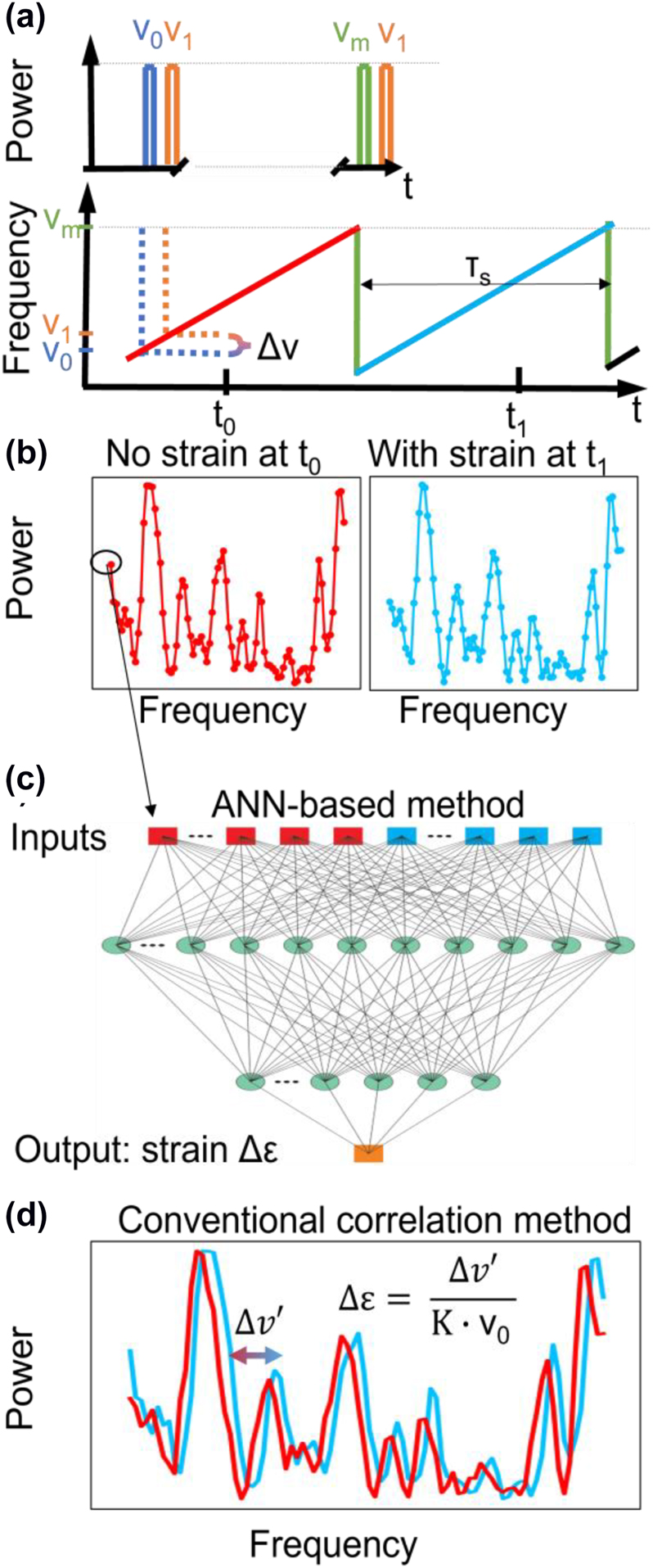
Schematic representation of the data obtained from the WS-COTDR and comparison of the conventional correlation-based approach and ANNs. (a) Sequential pulse generation of frequencies between v 0 and v m with step Δv during time periods of T s. The signal for the frequency modulation is given by a sawtooth function. (b) Backscattered power signatures resulted from two time periods with and without applied strain (illustrated in blue and red, respectively). (c) and (d) Signal processing of the two traces for strain change estimation using ANNs and the conventional correlation-based algorithm.
2.1.1 Signal processing based on conventional correlation algorithm and ANNs
Figure 1 illustrates the working principle of the WS-COTDR and how strain is extracted using the conventional approach based on correlation analysis and that of ANNs. First, a wavelength scan using m frequencies is performed when the fiber is free of strain at time t 0. The minimum and maximum frequency pulses are depicted in blue and green, respectively (Figure 1(a)). That measurement (red power signature) works as a reference. If strain is applied at time t 1, then a second scan will result in different backscattered powers for every frequency (light blue). As observed in Figure 1(d), the second trace at t 1 is shifted towards higher frequencies. The machine learning approach includes the use of ANNs which have as inputs the two traces and as an output a single strain value. The ANN architecture, shown in Figure 1(c) consists of two fully connected hidden layers with 1400 and 40 nodes in the first and second layer, respectively. The conventional approach, on the other hand, extracts strain by using Eq. (1):
where Δv′ and K are the strain-induced frequency shift extracted from a least mean square correlation algorithm and the fiber’s strain coefficient, respectively. More details about the correlation algorithm can be found in [35]. As can be seen in the example of Figure 1 the two traces are not identical due to the noise factor and the usage of the correlation algorithm can be cumbersome (especially in circumstances when noise levels are high). ANNs enable much faster signal processing and in contrast to the conventional approach, allow for real-time strain estimation. Apart from this, as presented later in Section 2.2.3, ANNs are more tolerant to noise and enhance the performance of the system providing more accurate strain results and expanding the measurement range.
2.1.2 Data and ANN training process
The ANN is trained using synthetic data and validated and tested on experimental data. The synthetic data consists of four million sweep pairs, similar to the red and light-blue traces in Figure 1, with one trace being the reference with zero strain change and the other one corresponding to a strain change. The strain values in the train dataset are uniformly distributed in the range of −200 nε to 200 nε. Furthermore, noise forming a gaussian distribution with mean equal to zero and standard deviation σ = 0.02 is added to the ideal synthetic data to combat overfitting and facilitate the algorithm to generalize [61]. We note that both the size of the train dataset and the noise standard deviation σ are optimized after a systematic study of their impact on the network’s performance.
The validation and test data are collected from experiments conducted in the lab using a standard optical fiber. The validation dataset corresponds to a fiber length of approximately 1 km, while the test dataset is obtained from measurement lengths of approximately 2 km and 5 km. Strain is applied on a section of approximately 14 m at the end of the optical fiber which is wound around a piezo tube. The piezo excites sinusoidal strain signals with amplitude 100 nε and frequency 20 Hz (validation dataset) and 28 Hz (test dataset). Figure 2 shows an example of the strain that the piezo applies to the optical fiber over time. The model’s performance is evaluated in terms of two key parameters, namely, the total harmonic distortion (THD) which represents the linearity of the sensor’s response and the strain amplitude spectral density (ASD) noise which is an indication of the system’s noise.
Temporal strain distribution along the fiber section wound around the piezo.
The schematic in Figure 3 depicts the whole training pipeline. Firstly, data are synthetically generated and experimentally collected. The synthetic data are used to train the model, which is validated after every training epoch (a pass through the whole training dataset) on experimental data. The validation performance is estimated after every epoch by the product of the two performance criteria, namely THD and ASD. At the end of the training phase (determined by the number of the epochs), the model with the best performance, defined as follows:
is stored.
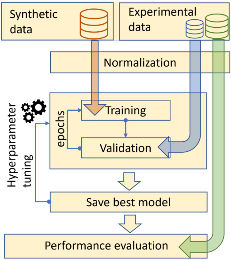
Training and model’s evaluation pipeline. Synthetic data are used for training, while experimental data are used for validation and testing. All data are normalized. During training, the algorithm passes through the train set many times, defined by the number of epochs. After every epoch, the ability of the model to generalize on experimental data (validation dataset) is examined. The model that arises from the training procedure is the one that performs best on the validation data as described in Eq. (2). This procedure is repeated systematically many times so that the algorithm’s hyperparameters are tuned. In the end, the model is evaluated on a different dataset (test data).
Part of the training process is also the hyperparameter tuning, which is performed by systematically tuning the hyperparameters’ values and evaluating their impact on the model’s performance P min. The hyperparameters then need optimization during the ANN training are related to the network’s architecture and the training algorithm. The size (number of nodes) and the number of hidden layers are among the most common structure-related hyperparameters and their optimized values are mentioned in Section 2.1 (two hidden layers with 1400 and 40 nodes, respectively). The hyperparameters that determine the learning, like the batch size and the learning rate are optimized at 1024 and 0.00003, respectively. Furthermore, a total number of 500 epochs is found to be enough to achieve the best performance (P min). After optimizing the hyperparameters, the model’s performance is finally evaluated on new and independent test data.
2.1.3 Performance evaluation of the ANN-assisted WS-COTDR
The ANN-assisted WS-COTDR is tested on data resulted from measurements up to approximately 1 km, 2 km and 5 km. The performance criteria are the already introduced THD and ASD noise. Table 1 summarizes the strain prediction performance of the correlation-based WS-COTDR and the ANN-assisted WS-COTDR. We observe that the ANNs outperform the correlation-based approach achieving lower ASD noise and THD values. We note that the correlation approach fails when a 5 km fiber is used rendering the use of ANNs essential.
Comparison of the performance of the correlation based WS-COTDR and the ANN-assisted WS-COTDR in terms of ASD noise and THD for different measurement distances.
| Distance [km] | ASD noise in nε/√Hz | THD in % | ||||
|---|---|---|---|---|---|---|
| Correlation | ANN | Improvement | Correlation | ANN | Improvement | |
| 1 | 0.273 | 0.230 | 15.8% | 0.452 | 0.337 | 25.4% |
| 2 | 0.364 | 0.318 | 12.6% | 5.827 | 0.663 | 88.6% |
| 5 | – | 0.501 | – | – | 0.663 | – |
-
The most significant improvement is related to the computation time. Specifically, the process of one million input sweeps using the correlation algorithm and the trained ANN lasts 94 s and 0.353 s, respectively. This means that the ANN shortens the computation time by 269 times. We note that these results are achieved by using an NVIDIA Quadro P4000 8GB RAM graphic card.
We have shown that ANNs perform and generalize very well on new data. However, we note that ANNs are not capable of extrapolating. Therefore, the model is expected to perform well as long as the strain levels to be measured lie within the strain range of the training dataset. For practical applications, where high levels of strain are expected, the ANNs can be trained with a very large dataset including a wide range of strain levels.
2.1.4 ANN-assisted WS-COTDR for real-time road traffic monitoring
Above we mentioned that ANN is 269 times faster than the conventional approach, which could enable real-time measurements. However, this can only be achieved after an extra step in signal processing is optimized. In practice, the frequency scanning shown in Figure 1(a) is not linear, and thus a numerical linearization is required. Specifically, a Mach–Zehnder interferometer is used to acquire the actual frequency changes Δv for each pulse that are used to linearize the saw-tooth signal. This linearization process is also time-consuming and for the process of one million sweep pairs 33.21 s are needed. ANNs can also be implemented for the frequency sweep linearization and reduce its computation time by 272 times. Further information regarding the linearization problem is provided in [33].
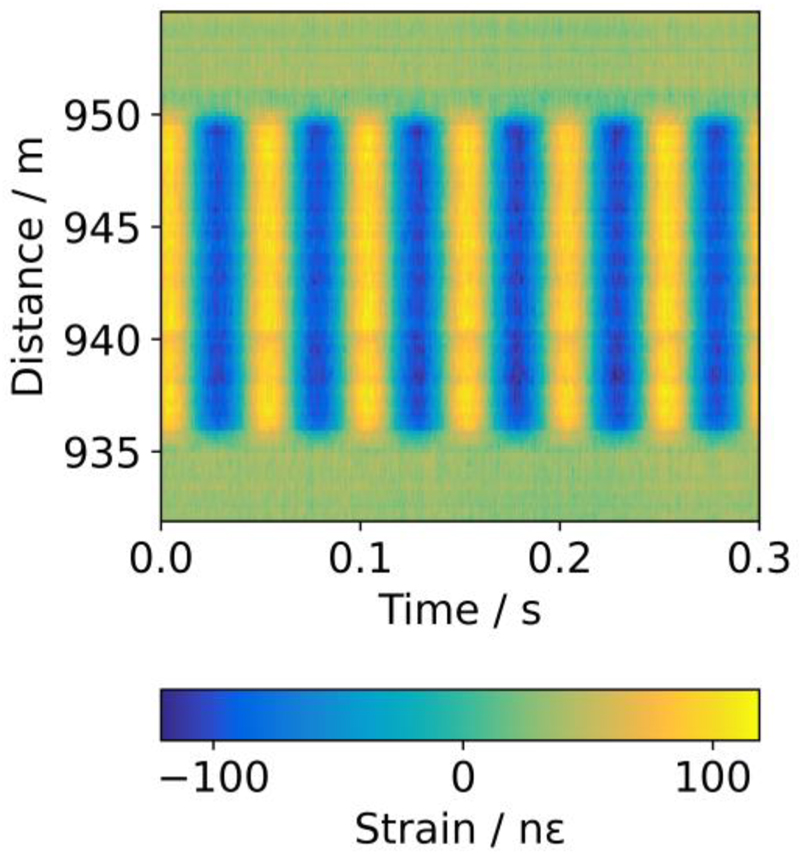
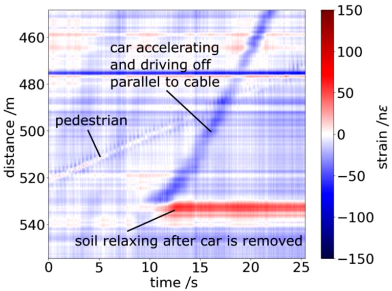
Signal processing using ANNs proved approximately 270 times faster than the conventional correlation-based signal processing. This potentially enables real-time strain estimation without storing raw data and opens the way for dynamic real-time and high-resolution strain (or vibration) monitoring in infrastructures using even the existing underground (dark) telecom fibers. As an example of the ANN-assisted WS-COTDR capabilities, we demonstrate near-surface strain monitoring (0.8 m depth) between two locations of our institute using a 1.3 km long dark fiber. The fiber is place at 5 m distance parallel to a car lane, and thus road traffic monitoring is feasible. Figure 4 shows the temporal soil deformation, calculated using the ANN-assisted WS-COTDR while a car is pulling out of a parking slot. The negative and the positive strain signature is attributed to the car weight and to the soil relaxation, respectively. From the linear negative signature, one could also estimate the car’s velocity, which in this case is approximately 30 km/h.
Distributed strain, calculated from raw data using the described ANNs, over time along fiber optic cable buried below sidewalk.
2.2 CNNs for spectra denoising and real-time ultra-long distance vibration sensing
Many applications require distributed fiber optic sensing over ultra-long km distances which is the case, for example in subsea power cable monitoring. However, the distance range of DFOS systems is limited by low signal-to-noise (SNR) data arising from distant backscattered signals [57]. This attenuation-limited distance range has been overcome to some extent by increasing the complexity and cost of the systems by employing additional hardware components [62, 63]. In this section we show how machine learning, and particularly CNNs can be used to denoise spectra and achieve up to 100 km sensing distance using an ultra-low loss optical fiber (Corning® SMF-28® ULL) [57]. The CNN-based denoising approach is applied to the ANN-assisted WS-COTDR system.
2.2.1 Architecture of the CNN denoiser
The data recorded using the WS-COTDR corresponding to a single time instance are two dimensional, with the axes being the sensing distance and the optical frequency. These two-dimensional data can be represented as images, which are the inputs of the CNN. Figure 5 shows a schematic of the complete CNN architecture starting from a noisy input and ending with the denoised output image. The CNN denoiser is characterized by a down and up sampling functionality as described in [64]. The noisy image undergoes a reversible down-sampling operation, which reshapes the image into four sub-images with a reduced number of pixels. The following CNN consists of a series of four layers with four filters each. We note that the first three layers are composed by a two-dimensional convolutional (Conv2D) and rectified linear units (ReLU) operations. The last convolutional layer is followed by an upscaling operator (reverse operator of the down-sampling operator applied to the noisy input image). In the end, the denoised image with the same number of pixels with the noisy input image is provided.
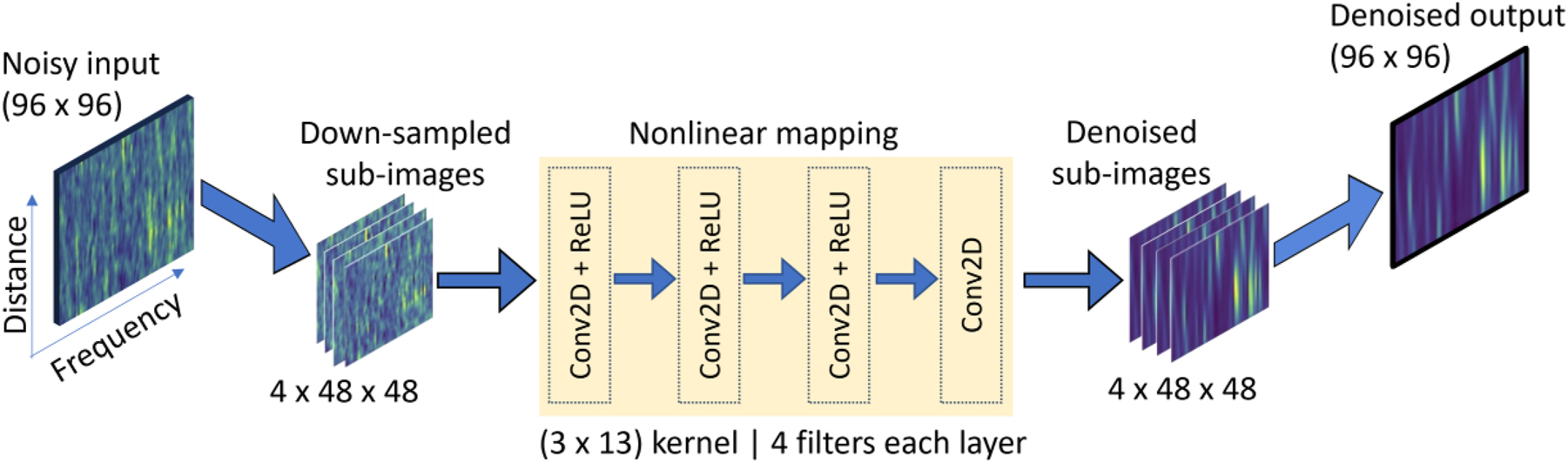
Architecture of the CNN-based denoiser.
2.2.2 Data and CNN training process
The training of the CNN is supervised, which means that a function that maps the input noisy images to the clean (ground truth) images is learnt from examples. So, the CNN is fed by pairs of noisy and clean images which are obtained by real measurements. The output images result from high SNR distributed measurements using up to 7 km fiber lengths while the noisy input images are the output images superimposed by noise. This noise results from measurements without a fiber connected to the system but using the system’s settings for ultra-long-distance operation. The noise added to the high SNR data is also multiplied by a noise factor, which is treated as hyperparameter during the CNN optimization. Therefore, noisy data similar to the ones obtained by actual ultra-long-distance measurements are generated.
Apart from the training dataset, validation and test datasets are needed for the validation and model’s evaluation, respectively. The validation dataset results from measurements over 100 km fiber length and is used to monitor the training process and save the model with the best performance in terms of strain error. Similar to the training pipeline, described in Figure 3, the validation dataset is also used to tune the hyperparameters. Among the most important hyperparameters are the learning rate, batch size and noise factor tuned at 0.00001, 16 and 4.5, respectively. We note that the structure of the CNN (number of convolutional layers, activation functions, down and up sampling conversion layers, filter and kernel size) shown in Figure 5 is also optimized in this training phase. The test dataset, used to evaluate the final model’s performance contains data from measurements along several fiber distances (70 km, 80 km, 90 km and 100 km).
In Figure 5 we observe that the images consist of 96 × 96 pixels. The number of pixels in the horizontal and vertical axis results from the optical frequencies used to perform a frequency sweep as illustrated in Figure 1 and the positions in the fiber defining the sampling resolution, respectively. Furthermore, we note that all measurements are conducted using a 10 Hz frequency sweep rate with pulse repetition rate equal to 1 kHz.
The evaluation of the image denoising performance is commonly performed by using algorithms such as peak signal to noise ratio (PSNR) [65] or the structural similarity index measure (SSIM) [66] but because the aim of the reported approach is to measure strain along very long fiber length, the most valid method to quantify the CNN performance is the estimation of the strain error when the denoised images are used. This necessitates applied strain levels on the optical fiber. In order to avoid unwinding and cutting the fiber at several positions and placing piezo stretchers, a strain-equivalent frequency shift modulation is applied. As already explained in Section 2.1, frequency shifts due to strain changes can be compensated by shifting the laser’s central wavelength. Therefore, a way to induce strain-equivalent shifts of the Rayleigh backscattered spectrum is to superimpose onto the laser current an additional sinusoidal laser current modulation. The frequency of the additional modulation is set to 2 Hz for the training and validation data and 1 Hz for the test data. The 2 Hz and 1 Hz modulation corresponds to strains amplitudes equal to 64 με and 67 με, respectively.
2.2.3 Performance evaluation of the CNN denoiser
The performance of the CNN denoiser is evaluated on the test data and in terms of mean strain amplitude error. Furthermore, the mean strain amplitude errors extracted by the CNN-denoised images are compared to those extracted by the raw data and by a state-of-the-art denoiser called block matching denoising algorithm BM3D [67]. The results are shown in Table 2. We observe that at distances up to 80 km both denoisers do not improve the sensor’s performance significantly and no need for denoising is needed. However, above 90 km both denoisers reduce the strain error with the CNN denoiser outperforming the state-of-the-art BM3D.
Comparison of the performance in terms of mean absolute strain error for low SNR data (raw data) and denoised data using the state of the art denoiser BM3D and the CNN denoiser.
| Distance [km] | Mean absolute strain error [nε] | ||
|---|---|---|---|
| Raw data | BM3D | CNN | |
| 70 | 0.46 | 0.57 | 0.03 |
| 80 | 1.85 | 0.87 | 0.18 |
| 90 | 23.1 | 6.93 | 0.37 |
| 100 | 53.84 | 34.59 | 5.61 |
We observe that the CNN denoiser performs well not only on data collected from the 100 km fiber but also on data with higher SNR collected from shorter fibers. This means that the CNN denoiser generalizes well and can potentially be used even if the data are not noisy. The strain level is not expected to significantly affect the performance of the CNN denoiser because the CNN is trained to simply denoise the spectra and not to extract strain. Therefore, the performance of the CNN depends mostly on the noise levels in the training dataset. However, the strain levels in the dataset affect the performance of the ANN models that are used to extract strain (Section 2.1).
Besides the significant performance improvement in terms of mean strain amplitude error, CNN denoiser is orders of magnitude faster than the BM3D. Specifically, the CNN denoiser processes a single 96 × 96 image in only 15.4 μs, while the BM3D denoiser requires 1.5 s. This potentially enables real-time denoising for fiber lengths up to approximately 128 km using the same measurement settings. It is of high importance to note that the computational times are calculated using an NVIDIA RTX 2080Ti graphic card.
2.3 ANNs for real-time train-tracking
In this section, we demonstrate how quite simple ANNs can be employed for efficient high-level processing of real-world DAS measurement data to be used for smart infrastructure monitoring. When compared to rule-based deterministic processing algorithms, the use of ANNs for measurement data processing can offer benefits in terms of processing speed or computational cost and enhanced input data ranges, thus improving adaptability to a broader range of conditions. In our example, noises and seismic vibrations induced by passing high-speed trains are monitored using a DAS system interrogating telecom fiber optic cables laid-out in parallel to the train tracks. The aim of processing these detected signals is to determine the current position and speed of running trains as precisely as possible and in real time.
2.3.1 Using DAS for train and railway monitoring
The idea to make use of trackside laid-out fiber optic cabling for DAS to enable train and track monitoring emerged in the last decade and has since garnered significant attention [28, 68–75]. Rail systems can be considered prime use cases for distributed fiber optic sensing based infrastructure monitoring due to their sheer extent and the broad range of possible application areas, e.g., network efficiency, security, and maintenance [34]. Furthermore, the almost ubiquitous availability of fiber optics alongside significant railroads and the increasing sensing range of available DFOS systems further facilitates this development. Concerning efficient railway operations, the need for accurate, real-time-capable localization of trains, the determination of corresponding velocities and permanent verification of train integrity (i.e., completeness) still is an important challenge [34]. In contrast to modern high-speed passenger trains, older trains and most of freight train traffic is not supported by GPS and/or other continuous positioning systems. Because of safety requirements like minimum safety distances between the trains, railroad networks are often operated below theoretical capacity due to the sparsity of existing train detection devices distributed along the tracks and the resulting coarse localization capabilities. The precise tracking of train movements continuously in time and distance minimizes the length of a railroad segment blocked by one train and increases the possible throughput of the network.
2.3.2 Signal characteristics
In Figure 6 an exemplary DAS recording along an approx. 35 km long segment of fiber optic cable laid out in parallel to railway tracks is depicted as a spatio-temporal waterfall plot. It exhibits the noises of two high-speed ICE trains running through the corresponding segment of the rail network. The inset presents a zoomed view, showing parts of the signal induced by the first train. The most obvious and distinguishable signal features aligned vertically correspond to the significant noises of consecutive bogie clusters of the passing train. These strong signal features can serve as support points for higher level measurement data processing (see below). When they are clear and distinguishable as in our example, they also provide a simple means to continuously check train integrity (i.e., completeness) irrespective of train velocity, since the number of cars (and thus the number of bogie clusters) is known for each train [28, 34].
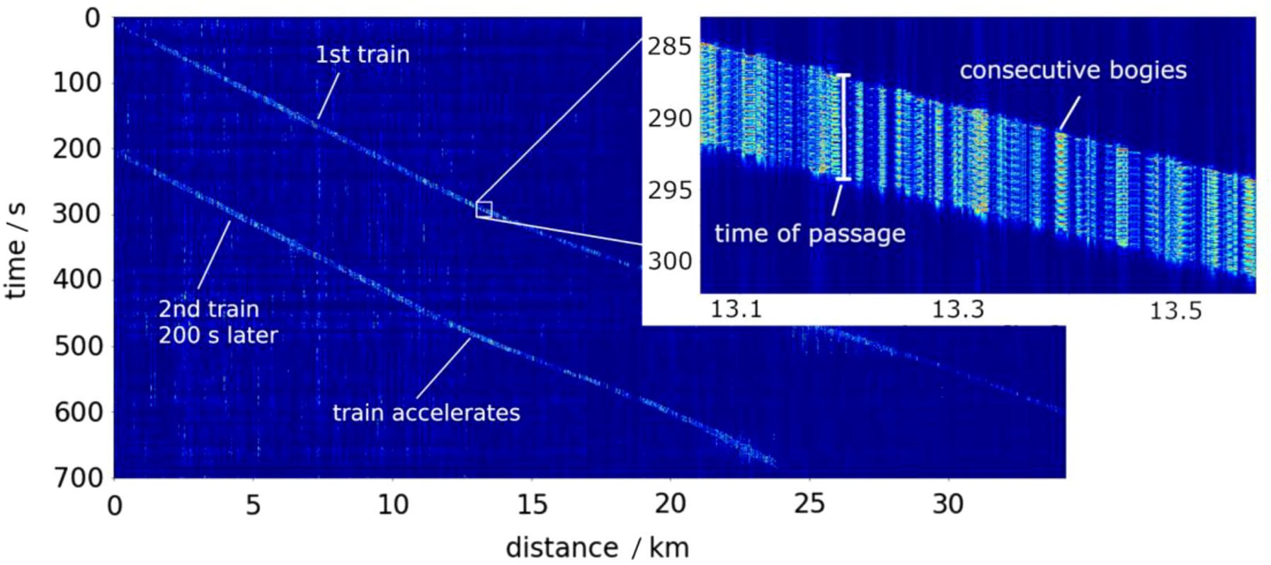
Waterfall diagram of DAS recording along an approx. 35 km long segment of trackside laid-out fiber optic cable showing noises from two successive high-speed ICE trains. The inset shows a zoomed view, with the width of the visible signal corresponding to the duration of passage of the entire train at a fixed position. Signal features aligned vertically exhibit distinguishable noises of individual bogie clusters of the train successively passing a position along the tracks.
Using DAS for continuous accurate and precise localization of trains faces significant challenges. For once, sensitivity of the DAS system differs along a given railway as the coupling of vibrations propagating from the track through the superstructure to the fiber optic cable heavily depends on the local conditions, e.g., the kind of the superstructure, the distance of the cable tunnel to the track or special environment like tunnels or bridges. This can result in blind spots or fiber segments with low SNR. Furthermore, environmental noises, e.g., from nearby road traffic or industry can degrade signal quality as they interfere with signals coming from passing trains. These issues and the diversity of environmental conditions faced with in the real world significantly complicate the accurate determination of the trains’ position and speed. Moreover, the enormous data throughput of modern DAS systems makes real time analysis extra challenging. In order to enable real time analysis of large noisy railway vibration data, a multitude of data treatment algorithms have been investigated in the literature [76, 77]. Apart from conventional rule-based algorithms, a promising way to fast analysis of DAS signals are ANNs. ANNs have been applied for pattern recognition and event classification tasks, such as identifying environmental noises like construction work next to tracks [78, 79]. Their use in DAS data processing algorithms can also significantly speed up the data treatment process [33]. Besides improving performance parameters like processing speed or broadening input data ranges, ANNs can also be used for speed analysis to be more robust, i.e., to generalize better among diverse conditions and local or temporary particularities in the obtained DAS signals. In the following we describe a simple ANN-based approach to efficiently obtain the train velocity from DAS-data and compare its working with a deterministic conventional algorithm.
2.3.3 Conventional and ANN-based data processing
To analyze DAS data with regard to train velocity, corresponding signals at different locations are shift-adjusted and centered in the same time window of train passage along all positions along the railway stretch as a pre-processing step. This produces what has been called the “rail-view” of a passing train [28–30]. The width of the resulting stripe then directly corresponds to the duration of passage of the train at a given position along the railway track, from which, together with the known train length, the velocity can be calculated. The horizontal lines stem from aligning the strong signals induced by the successive bogie clusters. Acceleration and deceleration of the train manifest themselves by a narrowing and widening of the train’s signal at a specific location, respectively, corresponding to a shorter or longer time of passage, respectively.
From the coarsely aligned rail view the train speed can be determined by further treating the pre-processed data using a deterministic algorithm based on finding narrow peaks in the signal or by direct processing utilizing a trained ANN.
For the pre-processing, the train noises are shifted such that the train’s signal is roughly centered in a 20 s time window. This is done by detecting the center of the passing train’s signal using a filter. Additionally, the train’s signal is normalized at each spatial position.
For the velocity analysis approach based on a deterministic algorithm, a most precise result hinges on the appropriate centering of the signal at each spatial position. To that end, a narrow peak finder is used to detect signals from specific bogie clusters (e.g., the most central ones) to finer align the rain signals using the bogies’ noises as support points. This requires a continuously high SNR in the noises of a set of at least a few bogie clusters of a given train. After that, filtering and sliding averaging in time and space is performed to smoothen the resulting rail-view [29]. Figure 7 shows an exemplary DAS signal of an ICE high-speed train in rail view format after the above was executed. The apparent high SNR signal of the train results from the high speed and weight as well as from adequate sensitivity of the DAS system along the railway segment under investigation. This, in turn, leads to high-quality velocity data for this measurement, as shown in Figure 9 (red curve). Nonetheless, one major drawback of the peak-finder data analysis used here is the need for manual tuning of the peak finding threshold parameters, like minimum peak height and peak width. These parameters differ for different types of trains and can also vary from one railway stretch to another. Moreover, the algorithm is comparably complex, and the resulting computational load will impede real-time analysis.
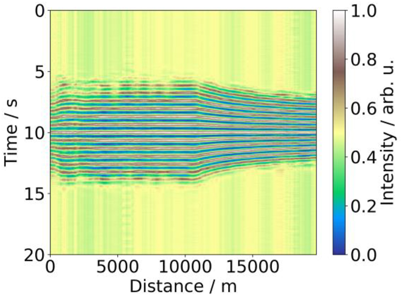
DAS signal of a single high-speed train along a 20 km railway stretch. The train noises have been shifted in time so that the train signal is centered within the shown 20 s interval. A peak-finding algorithm is used to fine-tune the shifts at each spatial position. The resulting shifted signal is normalized at each position and afterwards smoothed by employing a moving average in spatial and temporal direction, respectively.
A step towards train velocity determination from DAS data that is robust enough to adapt to different types of train and different tracks and railroad environments and fast enough for real-time analysis, is using a machine learning-based algorithm. In general, machine learning algorithms can be adapted to range of different conditions by providing it with real measurement data or synthesized data to be used for training the algorithm. Here, we have used an ANN with a simple architecture with seven fully connected hidden layers of 2048, 1024, 256, 128, 32, 8 and 2 neurons respectively. As input, it is designed to take a 20 s sample time trace at a given spatial position of the rail-view transformed data to predict from it the train speed as its sole output. As training data, we used synthetic DAS data resembling real train noises at a range of different velocities, as shown in Figure 8. This way, the input data range in terms of train speeds can be easily adjusted.
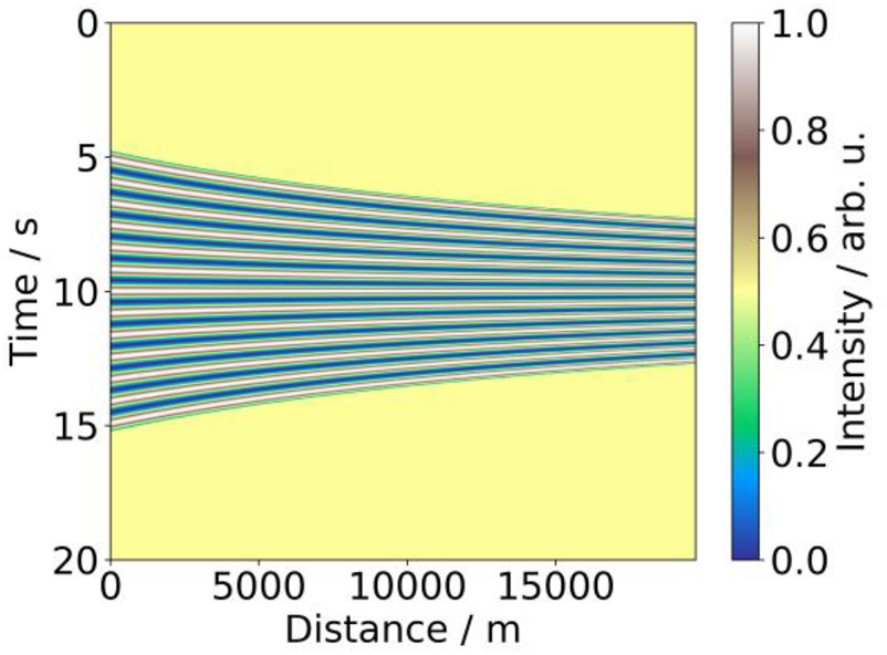
Synthetic DAS signals in rail view format corresponding to train noises at different velocities used as training data for the used ANN.
Figure 9 (green curve) depicts the determined velocity result of this simple ANN. It is obvious that its speed predictions are close to but not as precise as the results from applying the conventional peak finder algorithm. Nevertheless, the ANN’s performance is promising because it works with a wider velocity range and provides a much higher processing speed than the deterministic algorithm. Future upgrades of the ANN algorithm, e.g., by training it using both synthetic and real training data could improve its performance. Training the ANN with data from recordings of many trains, with specific characteristics of a given railway segment can also be included without having to tune parameters of rule-based peak finding algorithm by hand.
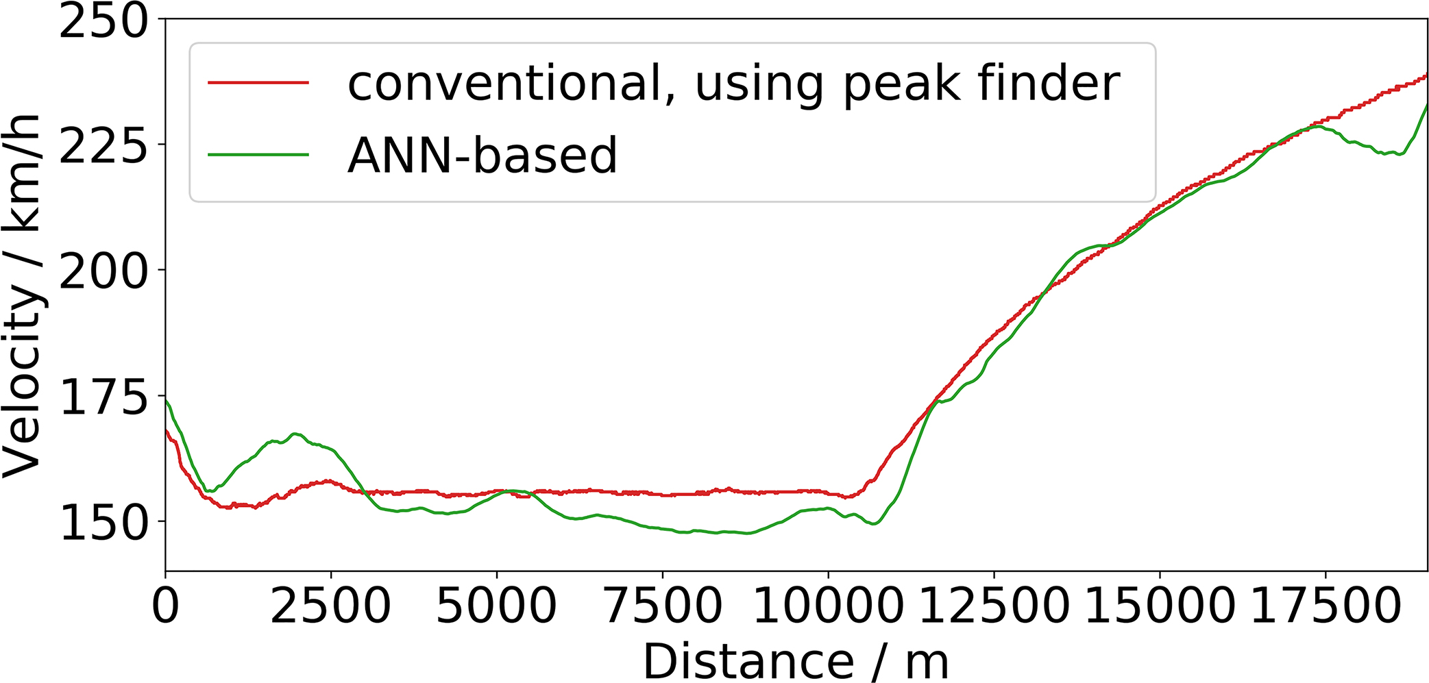
Comparison of determined location-dependent train velocities from DAS data corresponding to Figure 7. Compared are the cases of employing a rule-based (“conventional”) approach using a peak finder to identify the bogies’ signals (red curve) and utilizing the ANN-based algorithm (green curve), respectively.
3 Machine learning assisted Brillouin-based DFOS
3.1 CNNs for time-efficient long-range static temperature sensing
Brillouin optical frequency domain analysis (BOFDA) is among the most well-established techniques for static temperature and strain distributed fiber optic sensing [80]. A BOFDA system can reach approximately 60 km measurement length and achieve high spatial resolution on cm and even on mm range [25, 81, 82]. Ultra-long distance BOFDA sensing up to 100 km using Raman amplification has also been reported [26]. However, the relatively low cost is the characteristic that differentiates BOFDA from other Brillouin-based fiber optic sensors (e.g., Brillouin optical time domain analysis (BOTDA)) [25]. The low cost is attributed to the system’s interrogator that does not require expensive fast electronics [80]. Similar to BOTDA, the BOFDA signal is usually undergone a few averages during measurements in order to acquire spectra characterized by high SNR, which, in turn, affects positively the system’s performance in terms of temperature error [25]. However, the number of averages, as well as the measurement length have a negative effect on the system’s measurement time. In this subsection we show that CNNs deliver lower temperature errors than the conventional approach based on Lorentzian curve fitting (LCF) when faster measurements with low SNR are conducted. This shows that CNNs are more tolerant to noise and can potentially open the way for applications where fast monitoring and low errors are essential.
3.1.1 BOFDA sensing using conventional and CNN-based signal processing
BOFDA is a distributed fiber optic sensing technique based on stimulated Brillouin backscattering. Brillouin scattering is initiated by the pump waves travelling down the optical fiber and the acoustic phonons of the medium. This scattering is inelastic, and thus the frequency of the backscattered waves is shifted by Δf B, which is conventionally called Brillouin frequency shift (BFS). As mentioned, BOFDA is based on stimulated scattering, which means that the scattering effect is stimulated by injecting additional counterpropagating (Stokes) waves from the other end of the fiber with frequency equal to the expected Brillouin backscattered waves. We note that due to the damping ratio of the medium, a slight detuning between the Stokes and the Brillouin backscattered waves are still able to stimulate the backscattering and thus a typical Brillouin gain spectrum (BGS) is given as a function of Δf, which is the frequency difference between the incident pump and counterpropagating Stokes waves. The BGS is described by a Lorentzian curve, as follows [83]:
where w denotes the linewidth of the Lorentzian curve. The BFS (Δf B) is affected by changes in temperature and change and is conventionally extracted by performing LCF.
BOFDA provides distributed information of temperature and strain along optical fibers which is defined by the spatial resolution, which together with the measurement length, the number of Brillouin frequency tuning steps and the signal detection properties (namely the bandwidth and the number of signal averages) are related to the system’s measurement time. In this paper a 30-km optical fiber is measured with a spatial resolution set to 25 m and using six Brillouin frequency steps. The Bandwidth detection is set to 100 Hz and three signal averages are performed. These measurement parameters result in total measurement time of 4 min.
Figure 10 shows a typical BGS resulted from a 25 m segment of a 30 km long optical fiber and how this is analyzed using both the conventional and the CNN approach in order to acquire the temperature value corresponding to that segment. We note that the sampling rate is set to 16 which results in sixteen equally spaced BGS within the defined spatial resolution. While spatial resolution is set before conducting the measurements, the sampling rate adjustment belongs to the signal post processing. Details on how spatial resolution and sampling rate are set in BOFDA are given in [56].
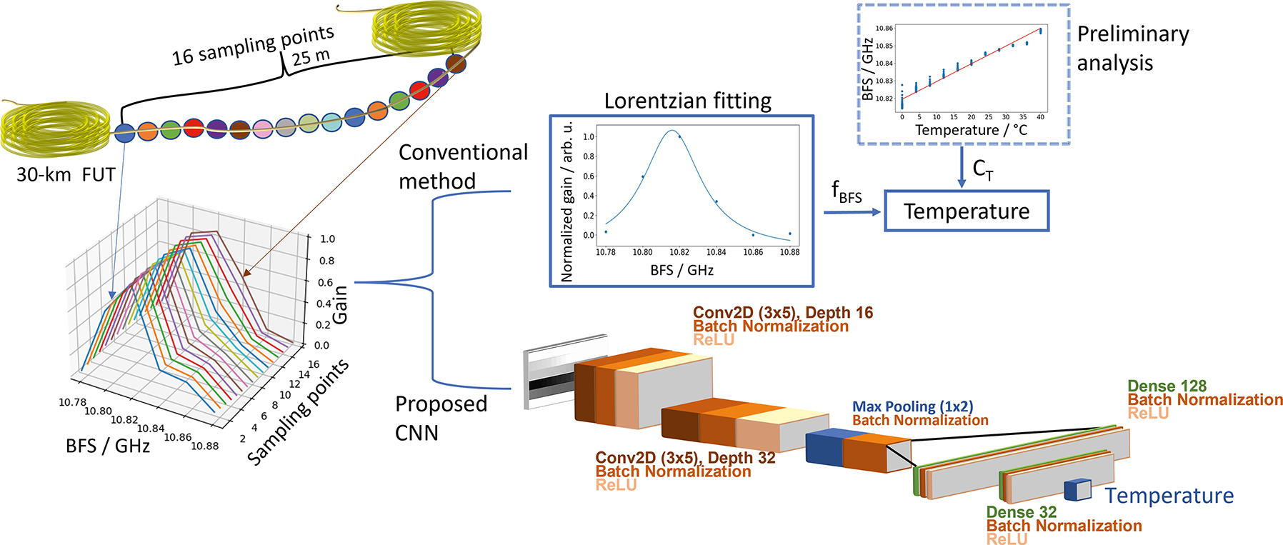
Schematic representation of the conventional and the CNN-based approach.
With the conventional approach, one performs LCF to every single BGS to estimate the BFS (Δf B). The performance of the LCF is related to the SNR and at distant positions, where the SNR decreases significantly, the BFS estimation becomes cumbersome and less accurate. Apart from the BFS, a preliminary analysis of the fiber under different temperature conditions is required to retrieve the temperature sensitivity of the fiber (C T). The BFS is linearly dependent on temperature and thus C T is estimated using linear fitting [80]. With the C T known, temperature can be extracted by any BGS. We note that the temperature extracted from the sixteen BGS is averaged.
The CNN-assisted BOFDA extracts temperature directly from the BGS without performing any curve fitting and any preliminary analysis. Nevertheless, training and hyperparameter optimization is required. The input of the CNN is an image 6 × 16 (Brillouin frequency steps × number of BGS) image being a two-dimensional representation of the BGS shown on the left side of Figure 10. The network’s architecture resembles that of the well-known VGG16, which is usually employed for image recognition in machine learning [84]. Two 3 × 5 convolutional layers are used with a depth of 16 and 32 for the first and second layer, respectively. After applying downsampling pooling, which works in one direction (1 × 2), the pooled feature map is flattened and two fully connected layers with sizes with 32 and 16 nodes, as shown in Figure 10 are used. The batch normalization layers are utilized to avoid overfitting [61] and alleviate the internal covariate shift [85]. The ReLU layers refer to the activation function which performs the nonlinear mapping [86].
The hyperparameters related to the algorithm itself are also optimized. Specifically, the required number of epochs, the batch size and the learning rate are 100, 64 and 0.001, respectively. We note that an NVIDIA RTX 2080Ti graphic card is used for training.
The CNN is trained, validated and tested using experimental data which are collected from measurements under different and controlled temperature conditions. Training and validation data were collected from an approximately 200 m segment placed at the beginning of the 30 km optical fiber. Specifically, 75% of that data are used for training and 25% for validation. The model is finally evaluated using test data collected for an approximately 200 m segment placed at the end of the 30 km optical fiber. The model is validated and tested according to the diagram in Figure 3 with the difference that the validation criterion being the validation loss, calculated in terms of square mean error instead of the P min as defined in Equation (2).
3.1.2 Performance evaluation of the CNN-assisted BOFDA
Figure 11 shows the mean temperature predictions (orange dots) on the test data using the LCF-based conventional approach and the CNN-assisted BOFDA in a range of temperatures from 0 °C to 40 °C. We observe that the CNN predictions are closer to the black dashed line that refer to the best-possible outcome predictions. Apart from the mean predictions, the prediction intervals corresponding to the standard deviation of the predictions are also illustrated in blue and manifest that the deviation of the CNN predictions is very low and varies significantly less than the LCF predictions at each set temperature. The total temperature absolute errors of the LCF and CNN-based approach are 3.5 °C and 1.7 °C, respectively. Because the test data arise from the segment at the end of the fiber, where the SNR is significantly lower, the CNN proves to be more tolerant against noise than the conventional LCF-based approach.
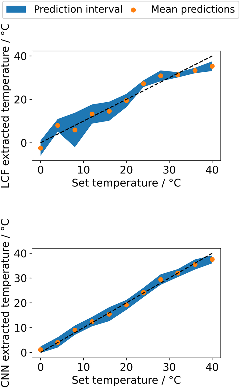
Mean temperature predictions using the LCF-based conventional approach (top) and the CNN (bottom), respectively. The mean temperature predictions are shown with orange dots while the prediction interval is illustrated in blue. The dashed lines represent the best-possible temperature predictions.
Although CNNs provide more accurate temperature predictions than the LCF approach on noisy data, the use of CNNs on data with high SNR is not beneficial. When high SNR spectra are obtained, the LCF is of high quality and the extraction of BFSs results in reliable temperature predictions, which cannot be improved further by CNNs. A study on the evaluation of the generalization performance of the CNN-assisted BOFDA shows that the usage of CNNs is advantageous in applications where long-range sensing is required [87].
The performance enhancement in terms of temperature error can also contribute towards shorter measurement times. The number of signal averages increases the SNR which can have a positive impact on the temperature errors but on the other hand increases the measurement time [56]. To estimate the improvement in measurement time that is achieved using CNNs, we examine the number of signal averages that are required to increase the SNR so that the conventional method can reach the temperature errors of the CNN-assisted BOFDA. This study is carried out, as an example, at 0 °C and shows that at least 27 averages are required which result in a total measurement time of 36 min. Therefore a nine-fold reduction in measurement time is achieved.
3.2 Machine learning algorithms for multiparameter sensing
In this section we show how machine learning can be used to simultaneously monitor temperature and humidity using BOFDA. In general, multiparameter Brillouin distributed sensing in not trivial due to the effect of cross-sensitivity [88, 89]. Specifically, both humidity and temperature affect the BFS, and thus the conventional method cannot decouple the two effects. To overcome this, a BOFDA setup characterized by a high SNR and assisted by machine learning algorithms is used.
3.2.1 Feature extraction and data acquisition
For simultaneous temperature and humidity sensing a polyimide-coated (PI) optical fiber (Fibercore SM1250(10.4/125)P) which is sensitive to both effects is used. Figure 12A shows a multipeak BGS of the PI-coated optical fiber (blue dots) retrieved by used our BOFDA system. This setup proved capable of recording a multipeak BGS, consisting of additional secondary peaks with amplitudes orders of magnitude lower than that of the fundamental peak. Furthermore, the multipeak LCF (red curve) fits almost perfectly with the experimental data. Together with the multipeak LCF, the individual Lorentzian components are also depicted (colored dashed curves). We note that the last peak is very broad indicating that two peaks are superimposed, and thus two Lorentzian components are used. The LCF is performed using the lmfit python library [90]. The quantities extracted from the LCF and used as features are the BFSs and linewidth of all the Lorentzian components. In total ten features are used.
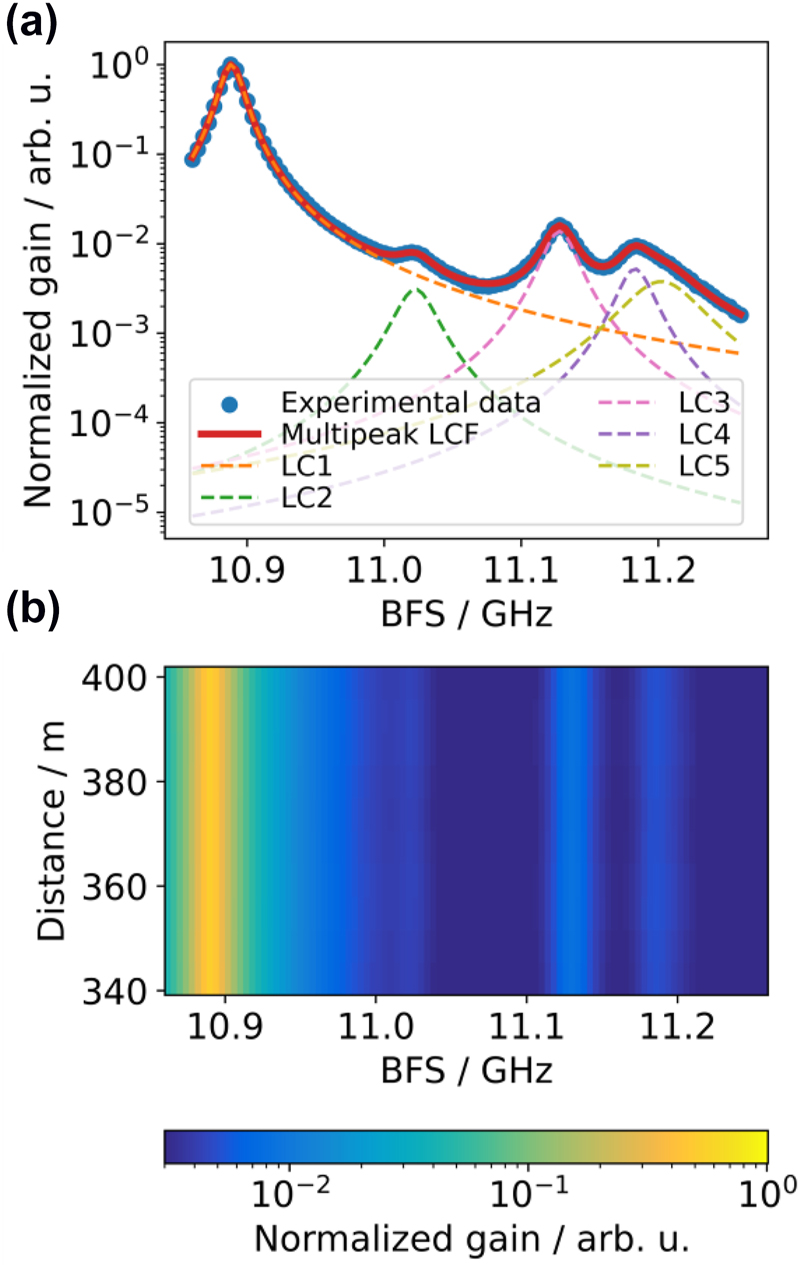
Measured multipeak Brillouin gain spectra. (a) Normalized logarithmic BGS at a random position along the FUT. Lorentzian curve fitting (LCF) is shown with a red curve while the Lorentzian components (LC) with colored dashed curves. (b) 2D representation of the normalized and logarithmic BGS from 340 m to 400 m.
Measurements are conducted along a PI-coated optical fiber of 400 m length. To regulate the temperature and humidity conditions, a segment of the fiber of approximately 60 m is placed in a climate chamber. A 2D representation of the BGS corresponding to this fiber segment is shown in Figure 12B. Since temperature and humidity conditions are the same along the optical fiber, we observe that the BGS is almost identical along at all positions. The temperature and humidity ranges are set from 40 °C to 60 °C and from 20%RH to 80%RH, respectively. At every set temperature and humidity condition, two distributed measurements along the optical fiber are conducted.
3.2.2 Performance evaluation of different machine learning algorithms for temperature and humidity discrimination
After extracting the BFSs and linewidths of all BGS using multipeak LCF we perform an exploratory data analysis. The scatter plot in Figure 13 shows, as an example, how the linewidth and the BFS of the fundamental peak change with relative humidity and temperature. We observe that while the BFS changes with both temperature and relative humidity, the linewidth depends solely on the BFS. Specifically, the BFS increases with temperature and relative humidity with coefficients equal to 1.1 MHz/°C and 100 kHz/%RH, respectively. Furthermore, we observe that the linewidth does not change linearly with temperature and the higher the temperature, the smaller the linewidth difference between two consecutive temperature steps. This manifests that nonlinear algorithms are more appropriate.
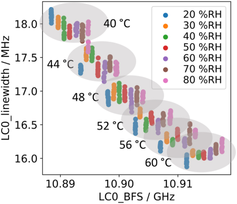
Scatter plot indicating how the linewidth and the BFS of the fundamental peak (LC0) vary with temperature and relative humidity.
Although in Figure 13 we show, exemplarily, the impact of temperature and relative humidity only on the BFS and linewidth of the fundamental peak, we make use of all the features extracted from the multipeak BGS. This results in 5 BFSs and 5 linewidths. First, a simple linear regression algorithm, which assumes only linear relations between the features and the target values (temperature and relative humidity) [91]. Even though the algorithm is very simple, it performs relatively well and manages to discriminate temperature and humidity providing absolute errors of 0.8 °C and 8.6%RH, respectively. To reduce the errors, more complex algorithms are applied. Polynomial regression works similarly with linear regression but makes use of features converted in their higher order terms [91]. Although polynomial regression can catch nonlinearities in the data, it becomes prone to overfitting when the order of polynomials increases. For this reason, L2 regularization is used. This kind of regression analysis is also known as ridge regression [91]. We find out that a second order polynomial reduces the humidity error by almost 1 °C. No significant change in temperature error is observed. Decision trees [92] are also utilized but only a slight decrease in humidity error is achieved. Specifically, we make use of an ensemble of five decision trees with depth and leaf nodes equal to 8 and 60, respectively. We note that these hyperparameters are optimized similarly to the optimization in ANNs, as shown in Figure 3. ANNs are employed, and they outperform all the previously used algorithms delivering a humidity error of 6.5%RH. The ANN consists of two hidden layers with 256 and 16 nodes in the first and second layer, respectively. The training is performed setting the batch size to 8 and the learning rate to 0.005. A comparison of the performance of all algorithms used is summarized in Table 3. We note that all the machine learning algorithms are applied using the Python scikit-learn library [93].
Comparison of the machine learning algorithms’ performances in terms of temperature and relative humidity mean absolute error.
| Algorithm | Mean absolute strain error | |
|---|---|---|
| Temperature in °C | Humidity in %RH | |
| Linear regression | 0.8 | 8.6 |
| Polynomial regression | 0.7 | 7.7 |
| Decision trees | 0.7 | 7.4 |
| ANNs | 0.9 | 6.5 |
The algorithms’ performance evaluation on temperature and humidity discrimination is estimated in this case using leave-one-out cross-validation. Due to the long measurement times, the number of the conducted distributed measurements along the optical fiber is limited, and thus there are not enough data that can be split into train, validation and test datasets. To make use of the whole dataset but also to get an unbiased prediction on unseen data, a kind of cross-validation is used. During cross-validation, N models are training using N − 1 distributed measurement excluding one measurement, which is used for testing. this approach is called leave-one-out cross-validation [94]. The errors shown in Table 3 are referred to the mean error of the N trained models. In the future more data will be collected, and the model will be evaluated not only in its ability to simply generalize on unseen data but also to interpolate and extrapolate out of the training range. A future work will also evaluate the model’s performance for applications in the field of structural health monitoring of infrastructures (e.g., long pipelines, subsea cable monitoring, corrosion detection) to examine its capabilities to adapt to new conditions [95].
The simultaneous measurements of temperature and humidity are time-consuming which is attributed significantly to the high SNR ratio that is required to obtain a clear multipeak spectrum which is characterized by secondary peaks whose amplitudes are more than two orders of magnitude lower than that of the fundamental peak (Figure 12). A future work will investigate the potential to use the CNN-assisted BOFDA which is very robust against noise (as described in Section 3.1) to discriminate temperature and humidity from measurements conducted in considerably shorter times.
4 Conclusions
We presented a few examples on how machine learning enhances the performance of dynamic (Rayleigh) and static (Brillouin) DFOS for applications in the field of infrastructure monitoring. Machine learning proved to be more tolerant against noise in both types of DFOS reducing considerably the temperature and strain errors. Moreover, in the case of the WS-COTDR (Rayleigh-based DFOS), the computation time to extract strain was reduced significantly by using ANNs. Specifically, the ANN approach proved to be 270 times faster than the conventional approach. This signal processing time is fast enough to potentially enable real-time dynamic strain monitoring. Applications of the dynamic DFOS systems in the field of road traffic and railway infrastructure monitoring were presented. CNNs were also used to extend the measurement length of the WS-COTDR and allow up to 100 km distributed sensing. In the case of BOFDA (Brillouin-based DFOS), the CNNs contributed significantly towards faster measurement times achieving a nine-fold time reduction in comparison to the classic system. Furthermore, machine learning was also used to address the well-known cross-sensitivity problem in DFOS and allow multiparameter sensing. In this case, temperature and humidity was measured simultaneously with errors equal to 0.9 °C and 6.5%RH. Therefore, the presented machine learning assisted DFOS can open the way towards a cost-effective distributed sensing for applications in long subsea cable monitoring and corrosion prevention in long pipelines.
Funding source: BAM PhD program
About the authors
Christos Karapanagiotis received the Diploma in Physics from the Aristotle University of Thessaloniki, Greece, and his M.Sc. degree in Optics and Photonics from the Karlsruhe Institute of Technology (KIT), Germany, in 2018. Currently, he conducts research at the Federal Institute for Materials Research and Testing (BAM), Germany, and his research interests include distributed fiber optic sensors and machine learning in non-destructive testing (NDT) applications.
Konstantin Hicke received his Diploma in physics from TU Berlin in 2009 and his PhD in physics from the University of the Balearic Islands (UIB), Palma, in 2014. His PhD thesis focused on nonlinear dynamics, chaos and synchronization effects in coupled semiconductor lasers and their usage for brain-inspired photonic data processing. He has been with BAM researching and developing fiber optic sensors since 2016. His current research interests include: distributed fiber optic sensing, distributed acoustic sensing (DAS), infrastructure and condition monitoring, large-scale hazard and threat detection using fiber optic sensing, and Machine Learning assisted fiber optic sensing.
Katerina Krebber studied physics and received the PhD degree in electrical engineering. She has more than 20 years experiences with the development of fibre optic sensors including distributed fibre optic sensors, FBG sensors, fibre optic radiation sensors and polymer optical fibre sensors. Since 2004 she has been with BAM. At BAM she is head of the Division Fibre Optic Sensors (BAM - Division 8.6 - Fibre Optic Sensors) and leader of a number of R&D projects. She is an author and a co-author of more than 200 scientific publications including 45 peer reviewed papers and book chapters, 120 proceedings papers, 25 invited and keynote lectures and patents. A comprehensive bibliography can be obtained from the BAM Publication Server PUBLICA.
Acknowledgements
We thank our partners in the projects “BLEIB” and “Monalisa” and at DB Netz AG for the great collaboration. We would further like to thank our colleagues Sebastian Chruscicki and Sven Münzenberger for the technical support.
-
Author contribution: All the authors have accepted responsibility for the entire content of this submitted manuscript and approved submission.
-
Research funding: C.K. acknowledges funding from the PhD program of Bundesanstalt für Materialforschung und -Prüfung (BAM).
-
Conflict of interest statement: The authors declare no conflicts of interest regarding this article.
References
[1] P. Lu, N. Lalam, M. Badar, et al.., “Distributed optical fiber sensing: review and perspective,” Appl. Phys. Rev., vol. 6, p. 041302, 2019. https://doi.org/10.1063/1.5113955.Search in Google Scholar
[2] C. M. Monsberger, P. Bauer, F. Buchmayer, and W. Lienhart, “Large-scale distributed fiber optic sensing network for short and long-term integrity monitoring of tunnel linings,” J. Civ. Struct. Health Monit., vol. 12, pp. 1317–1327, 2022. https://doi.org/10.1007/s13349-022-00560-w.Search in Google Scholar
[3] L. R. Jaroszewicz, N. Kusche, V. Schukar, et al.., “Field examples for optical fibre sensor condition diagnostics based on distributed fibre optic strain sensing,” in Fifth European Workshop on Optical Fibre Sensors, 2013.Search in Google Scholar
[4] C. Karapanagiotis, K. Hicke, A. Wosniok, and K. Krebber, “Distributed humidity fiber-optic sensor based on BOFDA using a simple machine learning approach,” Opt. Express, vol. 30, p. 12484, 2022. https://doi.org/10.1364/oe.453906.Search in Google Scholar PubMed
[5] Z. Qin, S. Qu, Z. Wang, et al.., “A fully distributed fiber optic sensor for simultaneous relative humidity and temperature measurement with polyimide-coated polarization maintaining fiber,” Sens. Actuators, B, vol. 373, p. 132699, 2022. https://doi.org/10.1016/j.snb.2022.132699.Search in Google Scholar
[6] P. Stajanca, K. Hicke, and K. Krebber, “Distributed fiberoptic sensor for simultaneous humidity and temperature monitoring based on polyimide-coated optical fibers,” Sensors, vol. 19, p. 5279, 2019. https://doi.org/10.3390/s19235279.Search in Google Scholar PubMed PubMed Central
[7] P. J. Thomas and J. O. Hellevang, “A fully distributed fibre optic sensor for relative humidity measurements,” Sens. Actuators, B, vol. 247, pp. 284–289, 2017. https://doi.org/10.1016/j.snb.2017.02.027.Search in Google Scholar
[8] C. He, S. Korposh, R. Correia, L. Liu, B. R. Hayes-Gill, and S. P. Morgan, “Optical fibre sensor for simultaneous temperature and relative humidity measurement: Towards absolute humidity evaluation,” Sens. Actuators, B, vol. 344, p. 130154, 2021. https://doi.org/10.1016/j.snb.2021.130154.Search in Google Scholar
[9] X. Lu, K. Hicke, M. Breithaupt, and C. Strangfeld, “Distributed humidity sensing in concrete based on polymer optical fiber,” Polymers, vol. 13, p. 3755, 2021. https://doi.org/10.3390/polym13213755.Search in Google Scholar PubMed PubMed Central
[10] E. Lewis, A. Wosniok, D. Sporea, D. Neguţ, and K. Krebber, “Gamma radiation influence on silica optical fibers measured by optical backscatter reflectometry and Brillouin sensing technique,” in Sixth European Workshop on Optical Fibre Sensors, 2016.10.1117/12.2236678Search in Google Scholar
[11] P. Stajanca and K. Krebber, “Radiation-induced attenuation of perfluorinated polymer optical fibers for Radiation monitoring,” Sensors, vol. 17, p. 1959, 2017. https://doi.org/10.3390/s17091959.Search in Google Scholar PubMed PubMed Central
[12] P. Stajanca, L. Mihai, D. Sporea, et al.., “Effects of gamma radiation on perfluorinated polymer optical fibers,” Opt. Mater., vol. 58, pp. 226–233, 2016. https://doi.org/10.1016/j.optmat.2016.05.027.Search in Google Scholar
[13] S. Rizzolo, A. Boukenter, Y. Ouerdane, et al.., “Distributed and discrete hydrogen monitoring through optical fiber sensors based on optical frequency domain reflectometry,” J. Phys.: Photonics, vol. 2, p. 014009, 2020. https://doi.org/10.1088/2515-7647/ab6a73.Search in Google Scholar
[14] Y. Lin, F. Liu, X. He, et al.., “Distributed gas sensing with optical fibre photothermal interferometry,” Opt. Express, vol. 25, p. 31568, 2017. https://doi.org/10.1364/oe.25.031568.Search in Google Scholar PubMed
[15] L. Schenato, “A Review of distributed fibre optic sensors for geo-hydrological applications,” Appl. Sci., vol. 7, p. 896, 2017. https://doi.org/10.3390/app7090896.Search in Google Scholar
[16] N. Nöther, A. Wosniok, and K. Krebber, “A distributed fiber optic sensor system for dike monitoring using Brillouin optical frequency domain analysis,” in Optical Sensors 2008, Bellingham, Washington, USA, SPIE, 2008, p. 700303.10.1117/12.775133Search in Google Scholar
[17] M. Nikles, “Long-distance fiber optic sensing solutions for pipeline leakage, intrusion, and ground movement detection,” in Fiber Optic Sensors and Applications VI, Bellingham, Washington, USA, SPIE, 2009, p. 731602.10.1117/12.818021Search in Google Scholar
[18] J. Tejedor, C. H. Ahlen, M. Gonzalez-Herraez, et al.., “Real field deployment of a smart fiber-optic surveillance system for pipeline integrity threat detection: architectural issues and blind field test Results,” J. Lightwave Technol., vol. 36, pp. 1052–1062, 2018. https://doi.org/10.1109/jlt.2017.2780126.Search in Google Scholar
[19] P. Stajanca, S. Chruscicki, T. Homann, S. Seifert, D. Schmidt, and A. Habib, “Detection of leak-induced pipeline vibrations using fiber—optic distributed acoustic sensing,” Sensors, vol. 18, p. 2841, 2018. https://doi.org/10.3390/s18092841.Search in Google Scholar PubMed PubMed Central
[20] P. Zhang, C. Liu, D. Yao, Y. Ou, and Y. Tian, “Multi-physical field joint monitoring of buried gas pipeline leakage based on BOFDA,” Meas. Sci. Technol., vol. 33, p. 105202, 2022. https://doi.org/10.1088/1361-6501/ac7bd6.Search in Google Scholar
[21] J. Prisutova, A. Krynkin, S. Tait, and K. Horoshenkov, “Use of fibre-optic sensors for pipe condition and hydraulics measurements: a review,” CivilEng, vol. 3, pp. 85–113, 2022. https://doi.org/10.3390/civileng3010006.Search in Google Scholar
[22] Y. Chung, W. Jin, B. Lee, et al.., “Towards efficient real-time submarine power cable monitoring using distributed fibre optic acoustic sensors,” in 25th International Conference on Optical Fiber Sensors, 2017.10.1117/12.2267474Search in Google Scholar
[23] A. Masoudi, J. A. Pilgrim, T. P. Newson, and G. Brambilla, “Subsea cable condition monitoring with distributed optical fiber vibration sensor,” J. Lightwave Technol., vol. 37, pp. 1352–1358, 2019. https://doi.org/10.1109/jlt.2019.2893038.Search in Google Scholar
[24] M. A. Graf, F. Ehmer, C. Eisermann, M. Jakobi, and A. W. Koch, “Faseroptische Überwachung von mechanisch deformierten Kabelgeflechtsstrukturen mittels optischer Zeitbereichsreflektrometrie/Fiber-optic monitoring of mechanically deformed cable structures by means of optical time-domain reflectometry,” TM - Tech. Mess., vol. 85, pp. s73–s79, 2018. https://doi.org/10.1515/teme-2018-0030.Search in Google Scholar
[25] T. Kapa, A. Schreier, and K. Krebber, “63 km BOFDA for temperature and strain monitoring,” Sensors, vol. 18, p. 1600, 2018. https://doi.org/10.3390/s18051600.Search in Google Scholar PubMed PubMed Central
[26] T. Kapa, A. Schreier, and K. Krebber, “A 100-km BOFDA assisted by first-order bi-directional Raman amplification,” Sensors, vol. 19, p. 1527, 2019. https://doi.org/10.3390/s19071527.Search in Google Scholar PubMed PubMed Central
[27] X. Lu, M. Schukar, S. Großwig, U. Weber, and K. Krebber, “Monitoring acoustic events in boreholes using wavelength-scanning coherent optical time domain reflectometry in multimode fiber,” in EAGE GeoTech 2021 Second EAGE Workshop on Distributed Fibre Optic Sensing, 2021, pp. 1–5.10.3997/2214-4609.202131010Search in Google Scholar
[28] G. Cedilnik, R. Hunt, and G. Lees, “Advances in train and rail monitoring with DAS,” in Optical Fiber Sensors, Washington D.C., USA, Optical Society of America, 2018, p. ThE35.10.1364/OFS.2018.ThE35Search in Google Scholar
[29] S. Kowarik, K. Hicke, S. Chruscicki, et al.., “Train monitoring using distributed fiber optic acoustic sensing,” in Optical Fiber Sensors Conference 2020 Special Edition, Washington D.C., USA, Optica Publishing Group, 2020, p. T3.25.10.1364/OFS.2020.T3.25Search in Google Scholar
[30] S. Kowarik, M. T. Hussels, S. Chruscicki, et al.., “Fiber optic train monitoring with distributed acoustic sensing: conventional and neural network data analysis,” Sensors, vol. 20, p. 450, 2020. https://doi.org/10.3390/s20020450.Search in Google Scholar PubMed PubMed Central
[31] D. Milne, A. Masoudi, E. Ferro, G. Watson, and L. Le Pen, “An analysis of railway track behaviour based on distributed optical fibre acoustic sensing,” Mech. Syst. Signal Process., vol. 142, p. 106769, 2020. https://doi.org/10.1016/j.ymssp.2020.106769.Search in Google Scholar
[32] K. Hicke, S. Chruscicki, and S. Münzenberger, “Urban traffic monitoring using Distributed Acoustic Sensing along laid fiber optic cables,” in EAGE GeoTech 2021 Second EAGE Workshop on Distributed Fibre Optic Sensing, 2021, pp. 1–3.10.3997/2214-4609.202131008Search in Google Scholar
[33] S. Liehr, L. A. Jäger, C. Karapanagiotis, S. Münzenberger, and S. Kowarik, “Real-time dynamic strain sensing in optical fibers using artificial neural networks,” Opt. Express, vol. 27, pp. 7405–7425, 2019. https://doi.org/10.1364/oe.27.007405.Search in Google Scholar
[34] A. Lämmerhirt, M. Schubert, B. Drapp, and R. Zeilinger, “Fiber optic sensing for Railways – Ready to use?!” in Signalling + Datacommunication, vol. 114, Hamburg, Germany, DVV Media Group, 2022, pp. 60–69.Search in Google Scholar
[35] S. Liehr, S. Münzenberger, and K. Krebber, “Wavelength-scanning coherent OTDR for dynamic high strain resolution sensing,” Opt. Express, vol. 26, p. 10573, 2018. https://doi.org/10.1364/oe.26.010573.Search in Google Scholar
[36] A. Wosniok, R. Jansen, L. Cheng, and S. Chruscicki, “Ortsaufgelöste Zustandsüberwachung von Brückenbauwerken mittels faseroptischer Sensoren,” in Tagungsband der DGZfP-Jahrestagung 2021, Deutsche Gesellschaft für Zerstörungsfreie Prüfung (DGZfP), 2021, pp. 1–8.Search in Google Scholar
[37] M. F. Bado and J. R. Casas, “A review of recent distributed optical fiber sensors applications for civil engineering structural health monitoring,” Sensors, vol. 21, p. 1818, 2021. https://doi.org/10.3390/s21051818.Search in Google Scholar PubMed PubMed Central
[38] P. Jousset, T. Reinsch, T. Ryberg, et al.., “Dynamic strain determination using fibre-optic cables allows imaging of seismological and structural features,” Nat. Commun., vol. 9, p. 2509, 2018. https://doi.org/10.1038/s41467-018-04860-y.Search in Google Scholar PubMed PubMed Central
[39] Z. J. Spica, M. Perton, E. R. Martin, G. C. Beroza, and B. Biondi, “Urban seismic site characterization by fiber-optic seismology,” J. Geophys. Res.: Solid Earth, vol. 125, no. 3, p. e2019JB018656, 2020. https://doi.org/10.1029/2019jb018656.Search in Google Scholar
[40] G. Fang, Y. E. Li, Y. Zhao, and E. R. Martin, “Urban near-surface seismic monitoring using distributed acoustic sensing,” Geophys. Res. Lett., vol. 47, no. 6, p. e2019GL086115, 2020. https://doi.org/10.1029/2019gl086115.Search in Google Scholar
[41] A. Sladen, D. Rivet, J. P. Ampuero, et al.., “Distributed sensing of earthquakes and ocean-solid Earth interactions on seafloor telecom cables,” Nat. Commun., vol. 10, p. 5777, 2019. https://doi.org/10.1038/s41467-019-13793-z.Search in Google Scholar PubMed PubMed Central
[42] M. R. Fernández-Ruiz, M. A. Soto, E. F. Williams, et al.., “Distributed acoustic sensing for seismic activity monitoring,” APL Photonics, vol. 5, p. 030901, 2020. https://doi.org/10.1063/1.5139602.Search in Google Scholar
[43] J. B. Ajo-Franklin, S. Dou, N. J. Lindsey, et al.., “Distributed acoustic sensing using dark fiber for near-surface characterization and broadband seismic event detection,” Sci. Rep., vol. 9, p. 1328, 2019. https://doi.org/10.1038/s41598-018-36675-8.Search in Google Scholar PubMed PubMed Central
[44] L. Shiloh, A. Eyal, and R. Giryes, “Deep learning approach for processing fiber-optic DAS seismic data,” in 26th International Conference on Optical Fiber Sensors, 2018.10.1364/OFS.2018.ThE22Search in Google Scholar
[45] P. D. Hernandez, J. A. Ramirez, and M. A. Soto, “Deep-learning-based earthquake detection for fiber-optic distributed acoustic sensing,” J. Lightwave Technol., vol. 40, pp. 2639–2650, 2022. https://doi.org/10.1109/jlt.2021.3138724.Search in Google Scholar
[46] A. Venketeswaran, N. Lalam, J. Wuenschell, et al.., “Recent advances in machine learning for fiber optic sensor applications,” Adv. Intell. Syst., vol. 4, p. 2100067, 2021. https://doi.org/10.1002/aisy.202100067.Search in Google Scholar
[47] N. Lalam and W. P. Ng, “Recent development in artificial neural network based distributed fiber optic sensors,” in 2020 12th International Symposium on Communication Systems, Networks and Digital Signal Processing (CSNDSP), 2020, pp. 1–6.10.1109/CSNDSP49049.2020.9249588Search in Google Scholar
[48] R. Ruiz-Lombera, A. Fuentes, L. Rodriguez-Cobo, J. M. Lopez-Higuera, and J. Mirapeix, “Simultaneous temperature and strain discrimination in a conventional BOTDA via artificial neural networks,” J. Lightwave Technol., vol. 36, pp. 2114–2121, 2018. https://doi.org/10.1109/jlt.2018.2805362.Search in Google Scholar
[49] B. W. Wang, L. Wang, N. Guo, Z. Y. Zhao, C. Y. Yu, and C. Lu, “Deep neural networks assisted BOTDA for simultaneous temperature and strain measurement with enhanced accuracy,” Opt. Express, vol. 27, pp. 2530–2543, 2019. https://doi.org/10.1364/oe.27.002530.Search in Google Scholar
[50] C. Karapanagiotis, K. Hicke, and K. Krebber, “Temperature and humidity discrimination in Brillouin distributed fiber optic sensing using machine learning algorithms,” in Optical Sensing and Detection VII, Bellingham, Washington, USA, SPIE, 2022, p. 121390R.10.1117/12.2620985Search in Google Scholar
[51] S. Liehr, “Artificial neural networks for distributed optical fiber sensing (Invited),” in 2021 Optical Fiber Communications Conference and Exhibition (OFC), 2021, pp. 1–4.10.1364/OFC.2021.Th4F.2Search in Google Scholar
[52] A. K. Azad, L. Wang, N. Guo, H. Y. Tam, and C. Lu, “Signal processing using artificial neural network for BOTDA sensor system,” Opt. Express, vol. 24, pp. 6769–6782, 2016. https://doi.org/10.1364/oe.24.006769.Search in Google Scholar PubMed
[53] Z. Y. Cao, N. Guo, M. H. Li, K. L. Yu, and K. Q. Gao, “Back propagation neutral network based signal acquisition for Brillouin distributed optical fiber sensors,” Opt. Express, vol. 27, pp. 4549–4561, 2019. https://doi.org/10.1364/oe.27.004549.Search in Google Scholar PubMed
[54] Y. Q. Chang, H. Wu, C. Zhao, L. Shen, S. N. Fu, and M. Tang, “Distributed Brillouin frequency shift extraction via a convolutional neural network,” Photonics Res., vol. 8, pp. 690–697, 2020. https://doi.org/10.1364/prj.389970.Search in Google Scholar
[55] Y. Yao and Y. Mizuno, “Neural network-assisted signal processing in Brillouin optical correlation-domain sensing for potential high-speed implementation,” Opt. Express, vol. 29, pp. 35474–35489, 2021. https://doi.org/10.1364/oe.439215.Search in Google Scholar PubMed
[56] C. Karapanagiotis, A. Wosniok, K. Hicke, and K. Krebber, “Time-efficient convolutional neural network-assisted brillouin optical frequency domain analysis,” Sensors, vol. 21, p. 2724, 2021. https://doi.org/10.3390/s21082724.Search in Google Scholar PubMed PubMed Central
[57] S. Liehr, C. Borchardt, and S. Münzenberger, “Long-distance fiber optic vibration sensing using convolutional neural networks as real-time denoisers,” Opt. Express, vol. 28, p. 39311, 2020. https://doi.org/10.1364/oe.402789.Search in Google Scholar
[58] H. Wu, H. Du, C. Zhao, and M. Tang, “24 km High-performance Raman distributed temperature sensing using low water peak fiber and optimized denoising neural network,” Sensors, vol. 22, p. 2139, 2022. https://doi.org/10.3390/s22062139.Search in Google Scholar PubMed PubMed Central
[59] H. Wu, Y. Wan, M. Tang, et al.., “Real-time denoising of brillouin optical time domain analyzer with high data fidelity using convolutional neural networks,” J. Lightwave Technol., vol. 37, pp. 2648–2653, 2019. https://doi.org/10.1109/jlt.2018.2876909.Search in Google Scholar
[60] G. Yang, K. Zeng, L. Wang, M. Tang, and D. Liu, “Integrated denoising and extraction of both temperature and strain based on a single CNN framework for a BOTDA sensing system,” Opt. Express, vol. 30, p. 34453, 2022. https://doi.org/10.1364/oe.469342.Search in Google Scholar
[61] X. Ying, “An overview of overfitting and its solutions,” J. Phys.: Conf. Ser., vol. 1168, p. 022022, 2019. https://doi.org/10.1088/1742-6596/1168/2/022022.Search in Google Scholar
[62] Z. N. Wang, J. J. Zeng, J. Li, et al.., “Ultra-long phase-sensitive OTDR with hybrid distributed amplification,” Opt. Lett., vol. 39, pp. 5866–5869, 2014. https://doi.org/10.1364/ol.39.005866.Search in Google Scholar
[63] L. D. van Putten, A. Masoudi, and G. Brambilla, “100-km-Sensing-range single-ended distributed vibration sensor based on remotely pumped Erbium-doped fiber amplifier,” Opt. Lett., vol. 44, p. 5925, 2019. https://doi.org/10.1364/ol.44.005925.Search in Google Scholar PubMed
[64] K. Zhang, W. Zuo, and L. Zhang, “FFDNet: toward a fast and flexible solution for CNN-based image denoising,” IEEE Trans. Image Process., vol. 27, pp. 4608–4622, 2018. https://doi.org/10.1109/tip.2018.2839891.Search in Google Scholar
[65] K. Egiazarian, M. Ponomarenko, V. Lukin, and O. Ieremeiev, “Statistical evaluation of visual quality metrics for image denoising,” in 2018 IEEE International Conference on Acoustics, Speech and Signal Processing (ICASSP), 2018, pp. 6752–6756.10.1109/ICASSP.2018.8462294Search in Google Scholar
[66] W. Zhou, A. C. Bovik, H. R. Sheikh, and E. P. Simoncelli, “Image quality assessment: from error visibility to structural similarity,” IEEE Trans. Image Process., vol. 13, pp. 600–612, 2004. https://doi.org/10.1109/tip.2003.819861.Search in Google Scholar PubMed
[67] K. Dabov, A. Foi, V. Katkovnik, and K. Egiazarian, “Image denoising by sparse 3-D transform-domain collaborative filtering,” IEEE Trans. Image Process., vol. 16, pp. 2080–2095, 2007. https://doi.org/10.1109/tip.2007.901238.Search in Google Scholar PubMed
[68] N. Duan, F. Peng, Y. Rao, J. Du, and Y. Lin, “Field test for real-time position and speed monitoring of trains using phase-sensitive optical time domain reflectometry (Φ-OTDR),” Proc. SPIE, p. 91577A–91571.10.1117/12.2059188Search in Google Scholar
[69] S. Kepak, J. Cubik, P. Zavodny, et al.., “Fibre optic track vibration monitoring system,” Opt. Quant. Electron., vol. 48, pp. 1–10, 2016. https://doi.org/10.1007/s11082-016-0616-9.Search in Google Scholar
[70] W. Lienhart, C. Wiesmeyr, R. Wagner, F. Klug, M. Litzenberger, and D. Maicz, “Condition monitoring of railway tracks and vehicles using fibre optic sensing techniques,” in Transforming the Future of Infrastructure through Smarter Information: Proceedings of the International Conference on Smart Infrastructure and ConstructionConstruction, 27–29 June 2016, ICE Publishing, 2016, pp. 45–50.Search in Google Scholar
[71] R. Martinek, J. Nedoma, M. Fajkus, and R. Kahankova, “Fiber-optic bragg sensors for the rail applications,” Int. J. Mech. Eng. Robot. Res., vol. 7, pp. 292–295, 2018. https://doi.org/10.18178/ijmerr.7.3.292-295.Search in Google Scholar
[72] A. Minardo, G. Porcaro, D. Giannetta, R. Bernini, and L. Zeni, “Real-time monitoring of railway traffic using slope-assisted Brillouin distributed sensors,” Appl. Opt., vol. 52, pp. 3770–3776, 2013. https://doi.org/10.1364/ao.52.003770.Search in Google Scholar PubMed
[73] J. Nedoma, M. Stolarik, M. Fajkus, M. Pinka, and S. Hejduk, “Use of fiber-optic sensors for the detection of the rail vehicles and monitoring of the rock mass dynamic response due to railway rolling stock for the civil engineering needs,” Appl. Sci., vol. 9, p. 134, 2019. https://doi.org/10.3390/app9010134.Search in Google Scholar
[74] F. Peng, N. Duan, Y.-J. Rao, and J. Li, “Real-time position and speed monitoring of trains using phase-sensitive OTDR,” IEEE Photon. Technol. Lett., vol. 26, pp. 2055–2057, 2014. https://doi.org/10.1109/lpt.2014.2346760.Search in Google Scholar
[75] A. V. Timofeev, D. V. Egorov, and V. M. Denisov, “The rail traffic management with usage of C-OTDR monitoring systems,” Int. J. Comput. Electr. Autom. Control Inf. Eng., vol. 9, pp. 1492–1495, 2015.Search in Google Scholar
[76] M. He, L. Feng, and J. Fan, “A method for real-time monitoring of running trains using Ф-OTDR and the improved Canny,” Optik, vol. 184, pp. 356–363, 2019. https://doi.org/10.1016/j.ijleo.2019.04.112.Search in Google Scholar
[77] A. Papp, C. Wiesmeyr, M. Litzenberger, H. Garn, and W. Kropatsch, “A real-time algorithm for train position monitoring using optical time-domain reflectometry,” in 2016 IEEE International Conference on Intelligent Rail Transportation (ICIRT), IEEE, 2016, pp. 89–93.10.1109/ICIRT.2016.7588715Search in Google Scholar
[78] Z. Wang, H. Zheng, L. Li, et al.., “Practical multi-class event classification approach for distributed vibration sensing using deep dual path network,” Opt. Express, vol. 27, pp. 23682–23692, 2019. https://doi.org/10.1364/oe.27.023682.Search in Google Scholar PubMed
[79] Y. Shi, Y. Wang, L. Zhao, and Z. Fan, “An event recognition method for Φ-OTDR sensing system based on deep learning,” Sensors, vol. 19, p. 3421, 2019. https://doi.org/10.3390/s19153421.Search in Google Scholar PubMed PubMed Central
[80] D. Garus, K. Krebber, F. Schliep, and T. Gogolla, “Distributed sensing technique based on Brillouin optical-fiber frequency-domain analysis,” Opt Lett., vol. 21, pp. 1402–1404, 1996. https://doi.org/10.1364/ol.21.001402.Search in Google Scholar PubMed
[81] R. Bernini, A. Minardo, and L. Zeni, “Distributed sensing at centimeter-scale spatial Resolution by BOFDA: measurements and signal processing,” IEEE Photonics J., vol. 4, pp. 48–56, 2012. https://doi.org/10.1109/jphot.2011.2179024.Search in Google Scholar
[82] A. Minardo, A. Coscetta, E. Catalano, R. Bernini, and L. Zeni, “High spatial resolution physical and chemical sensing based on BOFDA,” in SPIE Optics + Optoelectronics, vol. 11028, Bellingham, Washington, USA, SPIE, 2019.10.1117/12.2519934Search in Google Scholar
[83] Y. Koyamada, S. Sato, S. Nakamura, H. Sotobayashi, and W. Chujo, “Simulating and designing brillouin gain spectrum in single-mode fibers,” J. Lightwave Technol., vol. 22, pp. 631–639, 2004. https://doi.org/10.1109/jlt.2003.822007.Search in Google Scholar
[84] K. Simonyan and A. Zisserman, “Very deep convolutional networks for large-scale image recognition,” arXiv preprint arXiv:1409.1556, 2014.Search in Google Scholar
[85] S. Ioffe and C. Szegedy, “Batch normalization: accelerating deep network training by reducing internal covariate shift,” in International Conference on Machine Learning, PMLR, 2015, pp. 448–456.Search in Google Scholar
[86] C. M. Bishop, “Neural networks and their applications,” Rev. Sci. Instrum., vol. 65, pp. 1803–1832, 1994. https://doi.org/10.1063/1.1144830.Search in Google Scholar
[87] C. Karapanagiotis, “Evaluation of the generalization performance of a CNN-assisted BOFDA system,” in Sensors and Measuring Systems; 21th ITG/GMA-Symposium, 2022, pp. 1–4.Search in Google Scholar
[88] C. Galindez, F. J. Madruga, and J. M. Lopez-Higuera, “Influence of humidity on the measurement of brillouin frequency shift,” IEEE Photon. Technol. Lett., vol. 20, pp. 1959–1961, 2008. https://doi.org/10.1109/lpt.2008.2005530.Search in Google Scholar
[89] F. Farahi, D. J. Webb, J. D. C. Jones, and D. A. Jackson, “Simultaneous measurement of temperature and strain - cross-sensitivity considerations,” J. Lightwave Technol., vol. 8, pp. 138–142, 1990. https://doi.org/10.1109/50.47862.Search in Google Scholar
[90] M. Newville, T. Stensitzki, D. B. Allen, M. Rawlik, A. Ingargiola, and A. Nelson, Lmfit: Non-linear Least-Square Minimization and Curve-Fitting for Python, 2016, Astrophysics Source Code Library, record ascl:1606.014, SAO/NASA Astrophysics Data System.Search in Google Scholar
[91] K. P. Murphy, Machine Learning: A Probabilistic Perspective, Cambridge, Massachusetts, USA, MIT Press, 2012.Search in Google Scholar
[92] S. Shalev-Shwartz and S. Ben-David, Understanding Machine Learning: From Theory to Algorithms, New York City, NY, USA, Cambridge University Press, 2014.10.1017/CBO9781107298019Search in Google Scholar
[93] F. Pedregosa, G. Varoquaux, A. Gramfort, et al.., “Scikit-learn: machine learning in Python,” J. Mach. Learn. Res., vol. 12, pp. 2825–2830, 2011.Search in Google Scholar
[94] Y. L. Zhang and Y. H. Yang, “Cross-validation for selecting a model selection procedure,” J. Econom., vol. 187, pp. 95–112, 2015. https://doi.org/10.1016/j.jeconom.2015.02.006.Search in Google Scholar
[95] P. Goodarzi, A. Schütze, and T. Schneider, “Comparison of different ML methods concerning prediction quality, domain adaptation and robustness,” TM - Tech. Mess., vol. 89, pp. 224–239, 2022. https://doi.org/10.1515/teme-2021-0129.Search in Google Scholar
© 2023 the author(s), published by De Gruyter, Berlin/Boston
This work is licensed under the Creative Commons Attribution 4.0 International License.
Articles in the same Issue
- Frontmatter
- Editorial
- Measurement systems and sensors with cognitive features II
- Research Articles
- Uncertainty-aware automated machine learning toolbox
- Explainable AI for sensor-based sorting systems
- Review Article
- Perspectives on AI-driven systems for multiple sensor data fusion
- Research Articles
- A collection of machine learning assisted distributed fiber optic sensors for infrastructure monitoring
- Automated end-of-line quality assurance with visual inspection and convolutional neural networks
- Review Article
- Automotive mass production of camera systems: Linking image quality to AI performance