Identification of consistent functional genetic modules
-
Jeffrey C. Miecznikowski
 ,
Daniel P. Gaile
,
Daniel P. Gaile

Abstract
It is often of scientific interest to find a set of genes that may represent an independent functional module or network, such as a functional gene expression module causing a biological response, a transcription regulatory network, or a constellation of mutations jointly causing a disease. In this paper we are specifically interested in identifying modules that control a particular outcome variable such as a disease biomarker. We discuss the statistical properties that functional networks should possess and introduce the concept of network consistency which should be satisfied by real functional networks of cooperating genes, and directly use the concept in the pathway discovery method we present. Our method gives superior performance for all but the simplest functional networks.
1 Introduction and objectives
It is often of scientific interest to find a set of genes that may represent an independent functional biological module or network, such as a functional gene expression module causing a biological response, a transcription regulatory network, or a constellation of mutations jointly causing a disease. This is in keeping with the modularity concept, where a module is a part of an organism that is integrated with respect to a certain kind of process and relatively autonomous with respects to other parts of the organism. The modularity concept has gained popularity more-or-less simultaneously in molecular biology and systems biology, developmental biology and evolutionary biology, and cognitive psychology (Wagner et al., 2007). The coordinated action of such sets of variables implies that the expressions or states of the module variables will be correlated. In addition, since the variables we are interested in are functional, their expression will correlate with the outcome variable y being studied. The identification of such modules can further the understanding of complex cellular mechanisms. In this article we will use the terms module, network and pathway interchangeably to refer to the same general concept. Although our discussion pertains to a variety of network element types, for definiteness of discussion we usually refer to the variables as genes.
An additional motivation for modeling pathways is that the power to detect important genes may be improved if the genes belong to the same module. In low signal-to-noise situations genes which are unidentifiable when evaluated individually may be discovered in a search for functional modules. The genes in a functional module may be identified by exploiting their mutual correlation and be seen as relevant in the context of a pathway or module.
We present three relevant properties a functional module should possess. The first two are the association of the module genes with each other, and the relationship of the module with the outcome variable. The third property is functional consistency, which relates the first two properties to more accurately describe real functional networks. We directly use this concept in the pathway discovery method we present. Previous approaches to pathway discovery that we discuss in this paper employ the first two properties in a sequential fashion, and do not address the third. The novel method of this paper introduces a method for identifying functional modules where co-expression and association with outcome are considered simultaneously, constrained by the consistency property.
We contrast our approach with two-step functional module-discovery approaches that incorporate information about co-expression (modularity) in one step and introduce gene-outcome association (functionality) information in a separate step. An example of a two-step method is the strategy of cluster analysis (modularity) followed by evaluating the identified clusters for the average correlation of the cluster members with the outcome variable (functionality). The functional information captured by the individual gene-outcome associations is not incorporated in the search for clusters at the first step. Much applied genomic analysis includes cluster analysis with subsequent study of the clusters. The basic approach can be implemented in a variety of ways by varying the similarity metric and the clustering method used, and has been extended and highly developed in Zhang and Horvath (2005) as part of a broad approach to network analysis they term Weighted Network Analysis (WNA).
In related work with a different objective, supervised principal components (SPC), Bair et al., (2006) finds components composed of genes which are predictive of outcome. In the first step SPC selects a set genes highly associated with outcome. Then principal components are computed for just those genes and the components are used for prediction. The number of selected genes is tuned using cross-validation to minimize the estimated out-of-sample prediction error using the principal component of the selected genes as the predictor. The components extracted by SPC are intended for prediction and not module identification. However, in the specific case that a single functional module influences the outcome, the genes selected would include the module genes and the principal component would load on the module genes which are mutually correlated, so it is natural to consider the use of SPC for functional module discovery. In that case, SPC would be an example of a two-step method which considers association with outcome in the first step and then co-expression in step two, the reverse order to the clustering approach.
Specifically in Section 2 we propose and justify a statistical model for functional gene networks. In Section 3 we propose methods to estimate the model and partition the eigenvalues. In Section 4 we discuss bagging techniques to improve the model estimation. In Section 5 we demonstrate our method and compare it with other methods via several simulations. In Section 6 we apply our methods to a simulated E. coli and S. cerevisiae datasets and a methylation dataset. We conclude the manuscript with a discussion and conclusion in Section 7.
2 Statistical model
2.1 Modularity
To represent modularity, we statistically represent gene co-expression by the correlation matrix of the gene expressions, and assume that there are groups of genes that are correlated among themselves while being uncorrelated with the other groups. Modularity implies a block structure for the appropriately ordered correlation matrix Σ. Note ordering here refers to the genes being collected or grouped into their associated pathways.
Let the vector x=(x1, x2, …, xN ) be gene expression variables which are measured independently on n individuals and let the data matrix be the n×N matrix X, so each row is the gene expression measurements for an individual (i.e. a gene expression array, xT). The form for the correlation matrix Σ is given by,
where Σjj is a nj ×nj within pathway correlation matrix, Δ is a d×d diagonal correlation matrix for a set D of independent genes which do not form modules, and
We assume that a within cluster correlation matrix Σjj arises from an independent module which can represent a biological pathway. A common simple pathway model is the single input module (SIM). We will use this model to depict common network properties and to construct simulation experiments.
2.1.1 Example: SIMs or Hub models
A SIM (Single Input Module) consists of a set genes that are controlled by a single transcription factor (Milo et al., 2002). There is considerable experimental evidence that SIMs occur frequently (Lee et al., 2002; Milo et al., 2002). For example, consider a SIM represented by the linear model for gene expression
where β>0, πi ∈{−1, 1} and the εi , i=0, 1, …, t are independent errors with mean 0 and variance
We model the functional aspect of the pathway by letting the hub x0 determine an outcome variable y by the regression function
where without loss of generality α>0. Letting the variance of the error term δ in (4) be
for a non-hub module gene xi .
A model SIM is depicted in Figure 1. The unfilled circle x0 indicates that it is unobserved, while the blue nodes are observed variables. The hub x0 represents the latent “driver” of the pathway and the arrow from x0 to y represents the influence of the module on y. In Figure 1, a negative sign on a link from x0 to xi indicates that a positive change in x0 which is associated with an increase in y suppresses xi , while a positive change indicates that xi is promoted.

The graph of a SIM. The consistency property is demonstrated by tracing paths between nodes.
2.2 A statistical definition of pathway
Three natural properties of an independent functional pathway or module are:
Modularity: The variables in a specific pathway are correlated with each other and independent of the variables in other modules. That is, we adopt the model (1) for the covariance matrix.
Functionality: Each pathway variable is marginally correlated with y.
Functional consistency: The pathway variables act in concert to either increase or decrease y. Given the pattern of covariation of the pathway variables, each variable causes y to change in the same direction – the pathway variables influence y in a consistent fashion.
Consistency requires a pathway to be a set of cooperating variables. For example, suppose the expression of a certain module gene promotes an increase in y while another gene in that module suppresses y. If the module is activated to increase y the promoter expression must increase while the suppressor decreases. Thus promoters and suppressors will be negatively correlated. The concept of consistency of functional effects is formalized in the following definition.
Definition: The effect of two variables xi and xj on y is functionally consistent when
if Cor(xi , xj ) is positive, then Cor(xi , y) and Cor(xj , y) have the same sign, and
if Cor(xi , xj ) is negative, then Cor(xi , y) and Cor(xj , y) have opposite signs.
Tracing paths in Figure 1 shows that a SIM has the consistency property. Path tracing rules in Wright (1934) imply that the correlation r between variables is calculated by multiplying the correlation assigned to the links on the paths joining them. For example, in Figure 1,
Lemma 1For any i≠j in a pathway, the number of negative elements in the set {Cor(xi , xj ), Cor(xi , y), Cor(xj , y)} is even.
Proof. Assume Cor(xi , xj ) is positive. Then consistent effect implies that either both Cor(xi , y) and Cor(xj , y) are positive or both are negative so the number of negative signs is 0 or 2. Alternatively, if Cor(xi , xj ) is negative consistent effect implies that exactly one of Cor(xi , y) and Cor(xi , y) is negative so the number of negative signs is 2.
Suppose that a potential pathway is being investigated for functionality. For example, after a cluster analysis the potential causal effect of a cluster on y is a typical question. The following theorem leads to a diagnostic measuring the conformity of that set of variables with the concept of consistent effect in Lemma 1.
Theorem 1Let X+be the set {xi :Cor(xi , y)>0} and X−be the set {xi : Cor(xi , y)<0}. Then consistent effect implies that
Cor(xi , xj )>0 when xi ∈X+ and xj ∈X+,
Cor(xi , xj )>0 when xi ∈X− and xj ∈X−,
Cor(xi , xj )<0 when xi ∈X+ and xj ∈X− or xi ∈X− and xj ∈X+.
Proof. The sign of Cor(xi , xj ) is determined according to the Lemma. □
Theorem 1 suggests a diagnostic to evaluate if a set of genes such as produced by a cluster analysis is varying consistently with respect to its association with y. Based on the association with y form the sets X+ and X− as in Theorem 1 and let X++={(i, j); i<j, xi ∈X+, xj ∈X+}, X−−={(i, j); i<j, xi ∈X−, xj ∈X−}, X+−={(i, j); xi ∈X+, xj ∈X−} and define the Consistency C to be
where C will be 1 when the x’s have perfectly consistent effects on y and will be –1 when consistency is violated to the maximum degree.
The main result of this paper is a pathway identification method which explicitly uses consistency to determine the set of genes satisfying our understanding of how a pathway should behave. To this end, we define a matrix W which captures our three criteria for a pathway, including consistency of effect. Define the cofunction matrixW as
where we add diag to denote that diag(Cor(x, y)) is a diagonal matrix with element i on the diagonal equal to Cor(xi , y). Note that elements of W are such that wij =Cor(xi , y)Cor(xj , y)Cor(xi , xj ). When both xi and xj are associated with y, Cor(xi , y)Cor(xj , y) will be of large magnitude – if each of them is in some functional pathway it will capture that. Likewise Cor(xi , xj ) will have large magnitude if xi and xj are in the same pathway. Then wij will be large when xi and xj are in the same functional pathway. To depict this, note that W can be written as
where the operator · denotes elementwise multiplication and 1N is an N×N matrix consisting of 1’s. The matrix to the left of · in (7) contains the information on the modular structure, while the matrix to the right of · in (7) is positive when the variables corresponding to that element are both associated with y. Figure 2 graphically depicts the formation of W for a fictitious set of simulated modules.
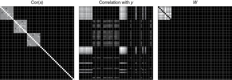
The formation of
Clearly W captures Property 1 since zeroes in Σ force zeros in W. By Property 2, modules in Σ which are not functional vanish from W. The third property implies that W is composed of positive elements, resembling a similarity matrix. To see this, recall that wij is of the form Cor(xi , xj ) Cor(xi , y) Cor(xj , y). By the lemma the number of negative factors is even so in a consistent pathway wij is non-negative. Thus to enforce consistency we transform negative elements of W to be zero.
By modularity W will inherit the block diagonal structure of Σ. In this article we assume that a single module is governing the variable y in the experiment. To discover the blocks (modules) of W we will estimate its eigenstructure.
2.3 Eigenanalysis
It is clear that if Wii is a block of W which when considered as a separate matrix has eigenvalue λi and eigenvector vi , the augmented vector
with vi in the position corresponding to block i, is an eigenvector of W with eigenvalue λi and so “picks out” the pathway when searching for the non-zero elements in the eigenvector.
Our model treats a module or pathway as a block of W with positive elements. A square block of dimension m which is approximated by μE where E is the m×m matrix of 1’s (so the block is approximately homogeneous) and μ>0 has one eigenvalue equal to μm and the rest equal to 0. That is,
The above considerations imply that the eigenvectors corresponding to the largest eigenvalues of W will identify the blocks of W and thus the pathways. Since the eigenvalue is a function of block size, larger modules will tend to have larger eigenvalues, as will modules with numerically larger elements in W (a function of the covariance of the genes with each other and with outcome). Thus the eigenanalysis will identify eigenvalues in decreasing order, so higher cardinality modules with stronger correlations and effect sizes will be found first.
We modify W in order to minimize the effect of functional genes which are not in a pathway and which operate independently of the other genes studied. Such a gene xi may be considered to be a block of size 1 with wij =1·cor(xi , y)2. The eigenvalue corresponding to this block is cor(xi , y)2 and the eigenvector will have 1 in the ith position and zeros elsewhere. We do not want to select these elements so we alter W to give them eigenvalue zero by using the modified matrix W0=W−diag(W), a common practice when defining an association matrix. Note diag(W) is a matrix with zeroes on the off diagonal and the diagonal elements of W on its diagonal. The eigenvalue of a valid size m functional pathway will change only slightly by a factor of
3 Estimation and partitioning the pathway eigenvector
To implement our method we substitute sample estimates (Pearson correlation) for the correlations forming W in (7). Theoretically the non-pathway elements of the first eigenvector of W0 will be zero, but of course this does not occur with real data. The eigenvector will be a mixture of two components: the elements corresponding to the pathway genes, and the remaining elements corresponding to non-pathway genes which we assume to be of smaller magnitude. One approach to partitioning the vector is choosing a mixture analysis method to partition the vector. Another approach would be to use a
4 Resampling approaches
We also introduce a resampling approach to compute a robust estimate of the eigenvectors of W0. Our approach is similar to a bagging approach. In bootstrap aggregation or “bagging” [see Breiman (1996)] we improve upon an unstable estimator for a given set of data. Bagged eigenvectors of W0 are obtained from an eigen-decomposition based on re-sampling entire rows from the original data with replacement so that the bootstrap sample is consistent with the original dimensions of the data matrix. The primary advantages of bagged eigenvectors are smaller variance (large effective sample size) and higher accuracy as a point estimate, at the cost of slower computation. In short, bagging is essentially a variance reduction method (Breiman, 1996). Another interpretation of the bagged estimate is as an approximate Bayesian posterior mean estimate (Hastie et al., 2009). It allows us to construct a small-sample estimator of the first eigenvector for the theoretical W0.
Two major shortcomings of the eigen-decomposition based on bootstrap samples are: (1) reflection, which is the arbitrary change in the sign of the eigenvectors; and (2) reordering where two or more eigenvalues have very similar magnitude (Jackson, 1995). In the latter case, eigenvectors obtained from bootstrap samples may come out altered in their order relative to that found from the original sample. Under either condition, it may lead to the false acceptance of the null hypothesis that eigen-vector coefficients are not significantly different from zero. In order to address these drawbacks, we propose the following algorithm. Note that we focus on the rank-1 approximation to the modified matrix W0 and the corresponding first eigenvector of the modified matrix W0 in order to identify one pathway.
Generate a bootstrap sample (X, y)*b with replacement of samples from the original data and calculate the matrix
For each matrix
Calculate the correlation
Find
Inspect the sign of
Aggregate the bootstrap estimates by computing the bootstrap mean
(9)Run k-means on v̅ assuming 2 clusters (k=2).
In the evaluations and simulations to follow, the standard eigenvector and the resampling version described here performed very similarly.
5 Simulations
We simulated each of 200 instances of (1) with 5 modules of 20 genes each and a set of 300 independent genes in Δ. The 5 modules are SIM’s, described by (2) and Figure 1. Only one of the modules is functional as per (4), the other four are uncorrelated with the outcome variable y. We set the model parameters to produce a specified signal-to-noise ratio (SNR) and intra-modular correlation rm . We defined SNR to be the ratio of ασε to σδ , that is, the square root of the ratio of the variance in y accounted for by the hub to the variance of the error component.
We compared our methods including clustering just the observed eigenvector (W.e) and clustering the bagged eigenvector (W.be), SPC, and three cluster analysis based methods. For supervised principal components we used the package superpc in R version 3.0.2 to calculate the first supervised principal component (Bair and Tibshirani, 2012). The clustering methods were k-means clustering using the data matrix X (K6), the partitioning around medoids algorithm (WGC6.r) using the absolute value of correlations of X (Pam.cor) and partitioning around medoids (PAM) using the correlations of X to the sixth power (WGC6.r6), which tends to differentially diminish small correlation coefficients with small magnitude. Note WGC6.r and WGC6.r6 are variants of Weighted Network Analysis (WNA) described in Horvath (2011). The clustering methods were set to obtain six clusters, the true number of clusters. However, in practice identifying the true number of clusters is difficult. The cluster analysis based methods computed the average significance for predicting y from the genes in each cluster (the module significance) and the functional module was taken to be the cluster with the highest module significance.
All methods are evaluated and compared in scenarios of coefficients with the same sign or random signs. In the simple case of coefficients with the same sign, we let πi =1 in (2) for all module genes, so that all intramodular correlations were the same sign. For a more general network of coefficients with random signs, we randomly selected each π from the set {−1, 1} so that a module could consist of a mix of promoters and suppressors.
For SNRs of 0.3 and 0.5 we calculated the average true positive rate (TPR) and the false discovery rate (FDR) for each method over 200 Monte Carlo simulations, for a range of intramodule absolute correlation (Rm) levels from 0.1 to 0.7. TPR was calculated as the average proportion of the true module genes selected by the method over our 200 Monte Carlo simulations. FDR is the average proportion of selected genes which actually are module genes. 200 Monte Carlo simulated samples were generated for each model for sample sizes of 100 and 300 and the averages of TPR and FDR over the simulations were calculated.
Figures 3 through 6 were generated using coefficients with the same sign. Figures 3 and 4 show results for case of constant coefficient sign and sample size of 100. In that setting, K6 outperformed all the other methods. When both TPR and FDR are taken into account the proposed methods W.e and W.be are preferred to all but K6. Note SPC performs the worst, which is not surprising since it is optimized for prediction and was not intended for module discovery. With the larger SNR value of 0.5, FDRs of the proposed methods and K6 start to stabilize around values below 0.05 at the intramodule absolute correlation level of 0.4. The remaining methods have unacceptable FDR. The same pattern holds for sample size 300 (Figures 5 and 6). At that sample size the proposed methods and K6 have FDRs below 0.05 when the intramodule absolute correlation level is 0.3 or greater for SNR is 0.3 (Figure 5) and for SNR=0.5 the FDR is close to 0 when the intramodule absolute correlation level is 0.2 or greater (Figure 6).

True positive rate and false discovery from simulation study with SNR of 0.3, a sample size of 100 and coefficients with the same sign. Rm is the magnitude of the correlation between module genes.
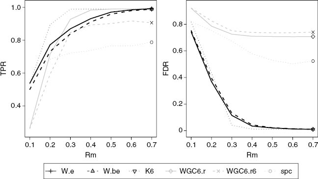
True positive rate and false discovery from simulation study with SNR of 0.5, a sample size of 100 and coefficients with the same sign. W.e and W.be are our basic and bootstrap pathway discovery method. K6, WGC6.r, and WGC6.r6 are variants of Weighted Network Analysis (WNA), using, respectively k-means for 6 clusters, PAM for 6 clusters using absolute correlation, and PAM for 6 clusters using correlation to the sixth power. SPC is Sparse Principal Components.

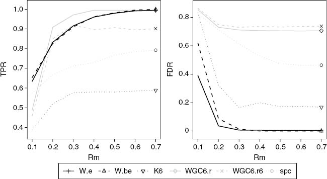
True positive rate and false discovery from simulation study with the SNR of 0.3, a sample size of 300 and coefficients with the same sign.

True positive rate and false discovery from simulation study with the SNR of 0.5, a sample size of 300 and coefficients with the same sign. W.e and W.be are our basic and bootstrap pathway discovery method. K6, WGC6.r, and WGC6.r6 are variants of Weighted Network Analysis (WNA), using, respectively k-means for 6 clusters, PAM for 6 clusters using absolute correlation, and PAM for 6 clusters using correlation to the sixth power. SPC is Sparse Principal Components.
When random signs are generated (Figures 7–10) the proposed methods outperform the remaining methods including K6. Although WGC6.r has higher TPR for Rm>0.2 it has a very high FDR and is not a competitor. K6 does very poorly in this scenario. We attribute the superiority of the proposed methods under varying directions of gene-gene association to the use of consistency in defining groups of genes. To investigate this, Table 1 shows the average functional consistency (5) over 100 simulations using the parameters of Figure 7, that is, SNR=0.3, a sample size of 100 and coefficients with random signs. We see that the proposed methods find more consistent modules except for the case of k-means which is most consistent. This seems surprising since k-means performed poorly in this situation (Figure 7). We attribute this to the fact that our k-means method uses Euclidean distance, while the correlation based clustering methods base distance on absolute correlation. Genes that vary inversely can be very highly correlated (small correlation-based distance) but tend to have large Euclidean distance. This is shown by plotting the distribution of the proportion of gene pairs with associations which are the dominant sign (positive or negative) for clusters picked up by k-means over 200 simulations with rm=0.3, SNR=0.3, and random sign (Figure 11). In our simulations, most of the selected genes by k-means have correlations of the same sign, which is consistent with small Euclidean distance. Thus k-means can only find subsets of the functional module, which results in the poor TPR shown in Figure 7.

True positive rate and false discovery from simulation study with the SNR of 0.3, a sample size of 100 and coefficients with random signs. W.e and W.be are our basic and bootstrap pathway discovery method. K6, WGC6.r, and WGC6.r6 are variants of Weighted Network Analysis (WNA), using, respectively k-means for 6 clusters, PAM for 6 clusters using absolute correlation, and PAM for 6 clusters using correlation to the sixth power. SPC is Sparse Principal Components.

True positive rate and false discovery from simulation study with the SNR of 0.5, a sample size of 100 and coefficients with random signs. W.e and W.be are our basic and bootstrap pathway discovery method. K6, WGC6.r, and WGC6.r6 are variants of Weighted Network Analysis (WNA), using, respectively k-means for 6 clusters, PAM for 6 clusters using absolute correlation, and PAM for 6 clusters using correlation to the sixth power. SPC is Sparse Principal Components.
True positive rate and false discovery from simulation study with the SNR of 0.3, a sample size of 300 and coefficients with random signs. W.e and W.be are our basic and bootstrap pathway discovery method. K6, WGC6.r, and WGC6.r6 are variants of Weighted Network Analysis (WNA), using, respectively k-means for 6 clusters, PAM for 6 clusters using absolute correlation, and PAM for 6 clusters using correlation to the sixth power. SPC is Sparse Principal Components.

True positive rate and false discovery from simulation study with the SNR of 0.5, a sample size of 300 and coefficients with random signs. W.e and W.be are our basic and bootstrap pathway discovery method. K6, WGC6.r, and WGC6.r6 are variants of Weighted Network Analysis (WNA), using, respectively k-means for 6 clusters, Pam for 6 clusters using absolute correlation, and Pam for 6 clusters using correlation to the sixth power. SPC is Sparse Principal Components.
Average consistency of modules detected.
| Methods | Rm=0.1 | Rm=0.2 | Rm=0.3 | Rm=0.4 | Rm=0.5 | Rm=0.6 | Rm=0.7 |
|---|---|---|---|---|---|---|---|
| K6 | 0.2339 | 0.3564 | 0.6479 | 0.8011 | 0.8602 | 0.8796 | 0.9064 |
| WGC6.r | 0.0978 | 0.1698 | 0.2613 | 0.3444 | 0.4121 | 0.4708 | 0.5206 |
| WGC6.r6 | 0.0981 | 0.1580 | 0.2356 | 0.3085 | 0.3740 | 0.4381 | 0.4843 |
| SPC | 0.2818 | 0.3291 | 0.3725 | 0.4068 | 0.4200 | 0.4464 | 0.4555 |
| W.e | 0.3096 | 0.4191 | 0.5585 | 0.6630 | 0.7081 | 0.7286 | 0.7370 |
| W.be | 0.3412 | 0.4213 | 0.5659 | 0.6795 | 0.7207 | 0.7349 | 0.7418 |

Distribution of proportion of dominant signs from modules found by k-means clustering.
To summarize, the proposed methods perform relatively well for all conditions and are clearly superior in the case of random signs, which represents a realistic biological network composed of both promoters and suppressors.
6 Examples
In this section we explore several examples. In the first example, we apply our methods to synthetic (simulated) datasets designed to simulate regulatory networks specific to specific organisms (e.g. S. Cerevisiae and E. coli). In the second example, we apply our methods to a methylation with gene expression dataset. In this way, we “connect the dots” between the data in Section 5 involving purely theoretical modules, to data simulating naturally occurring modules within an organism (e.g. yeast), to data where it is believed there is a biological connection between methylation and gene expression
The modular network models we have simulated certainly do not match the complexity of real microarray data. However, with real data the true underlying model is unknown so it is impossible to know which genes selected are true positives or misclassified irrelevant genes. To satisfy the criteria of realism and known properties, we generated datasets using SynTReN (Van den Bulcke et al., 2006) or Synthetic Transcriptional Regulatory Networks, a generator of synthetic gene expression data. This approach allows a quantitative assessment of the accuracy of the methods applied. The SynTReN generator generates a network topology by selecting subnetworks from the well characterized E. coli or S. cerevisiae regulatory networks. Then transition functions and their parameters are assigned to the edges in the network. Eventually, mRNA expression levels for the genes in the network are obtained by simulating equations based on Michaelis-Menten and Hill kinetics under different conditions (Chou, 1976). After the addition of noise, microarray gene expression measurements are produced.
We produced two synthetic expression datasets, one based on the E. coli network topology and one for S. cerevisiae. In each dataset there were 30 functional network genes and 300 background genes. The functional network was perturbed though an exogenous gene x0. The 300 background genes have an underlying network structure, but are not perturbed and so propagate only error. This is a more realistic model for inactive genes than in our simulations. We used the cluster addition option of SynTReN and set all parameters to their default values.
To introduce functionality we simulated y according to (4). We defined SNR to be the ratio of ασε to σδ . For SNRs ranging from 0.2 to 0.6, we calculated the average TPR and FDR for the same pathway detection methods as section 5 over 800 Monte Carlo simulations with a sample size of 400. Tables 2 and 3 show the results for the E. coli and S. cerevisiae organism, respectively. All of the methods except the proposed methods W.e and W.be have unacceptable FDR. Only WGC and WGC.6 have higher TPR but their FDR is over 80%. The proposed methods alone have FDRs in a range that allows them to be useful in practice. The results mirror the simulation in Section 5 with random signs, which suggests that the random sign model more accurately reflects real biological networks.
E. coli example.
| Measures | Methods | SNR=0.2 | SNR=0.3 | SNR=0.4 | SNR=0.5 | SNR=0.6 |
|---|---|---|---|---|---|---|
| TPR | K-means | 0.5092 | 0.5190 | 0.5290 | 0.5340 | 0.5423 |
| WGC | 0.7998 | 0.8026 | 0.8041 | 0.8044 | 0.8046 | |
| WGC.r6 | 0.8055 | 0.8104 | 0.8118 | 0.8120 | 0.8118 | |
| SPC | 0.4086 | 0.4836 | 0.5341 | 0.5568 | 0.5517 | |
| W.e | 0.6222 | 0.6214 | 0.6219 | 0.6222 | 0.6223 | |
| W.be | 0.6149 | 0.6204 | 0.6218 | 0.6221 | 0.6223 | |
| FDR | K-means | 0.8920 | 0.8894 | 0.8875 | 0.8869 | 0.8866 |
| WGC | 0.8579 | 0.8574 | 0.8572 | 0.8572 | 0.8571 | |
| WGC.r6 | 0.8585 | 0.8576 | 0.8573 | 0.8572 | 0.8572 | |
| SPC | 0.7841 | 0.7161 | 0.6629 | 0.6359 | 0.6131 | |
| W.e | 0.0787 | 0.0199 | 0.0041 | 0.0020 | 0.0000 | |
| W.be | 0.0593 | 0.0179 | 0.0031 | 0.0020 | 0.0000 |
S. cerevisiae example.
| Measures | Methods | SNR=0.2 | SNR=0.3 | SNR=0.4 | SNR=0.5 | SNR=0.6 |
|---|---|---|---|---|---|---|
| TPR | K-means | 0.4799 | 0.4875 | 0.4881 | 0.4885 | 0.4946 |
| WGC | 0.7886 | 0.7941 | 0.7930 | 0.7929 | 0.7914 | |
| WGC.r6 | 0.7889 | 0.7942 | 0.7934 | 0.7929 | 0.7929 | |
| SPC | 0.3895 | 0.4585 | 0.4548 | 0.4465 | 0.4448 | |
| W.e | 0.6239 | 0.6100 | 0.6071 | 0.6067 | 0.6067 | |
| W.be | 0.6069 | 0.6066 | 0.6067 | 0.6067 | 0.6067 | |
| FDR | K-means | 0.8836 | 0.8824 | 0.8819 | 0.8804 | 0.8804 |
| WGC | 0.8601 | 0.8590 | 0.8592 | 0.8593 | 0.8595 | |
| WGC.r6 | 0.8606 | 0.8596 | 0.8597 | 0.8597 | 0.8597 | |
| SPC | 0.8045 | 0.6990 | 0.6023 | 0.5314 | 0.4977 | |
| W.e | 0.0793 | 0.0218 | 0.0040 | 0.0000 | 0.0000 | |
| W.be | 0.0254 | 0.0035 | 0.0000 | 0.0000 | 0.0000 |
We also explore the ability to implement our techniques on two real datasets. The first dataset is designed to examine human adipose tissue markers via real time polymerase chain reaction (RT-PCR). The dataset is accessible at NCBI GEO database (accession number GPL19141) and contains 221 transcripts (genes) that encode proteins involved in metabolism, immune response, cell differentiation and proliferation, cell and tissue structure, transduction and response to stress. The study was designed to examine the effects of a longitudinal dietary intervention on human adipose tissue. It included 405 samples where the outcome variable was a factor variable that contained 3 levels, time at baseline in an 8 week diet (135 samples), at 8 weeks in an 8 week diet (135 samples), and at 24 weeks in an ad hoc maintenance diet (135 samples). Applying our method to this data with 200 bootstrap replications yields a functional pathway consisting of 8 genes. The heatmap for these 8 genes is shown in Figure 12. As expected it appears that each gene is functionally correlated with each other as well as with the outcome. Publications from the primary authors of this dataset (Viguerie et al., 2012) also cite several of the genes that we also discovered (e.g. SCD, LEP, ACSL1) as showing significant changes after the restricted diet. Specifically the stearoyl CoA desaturase (SCD) gene is cited as being a major hub gene and highly connected to components of the metabolic syndrome.

Adipose Tissue Data: Heatmap of the 8 genes in the functional pathway. The samples are arranged by outcome: Baseline, After 8 week diet, After weight maintenance diet. For purposes of the color mapping, the data are row normalized. The data support the functionality of the 8 gene pathway (similar profiles) and their correlation with outcome.
Our second example uses the The Cancer Genome Atlas (TCGA) urothelial bladder cancer (BLCA) dataset. Review of the literature pertaining to urine based methylation markers in bladder cancer suggests that HOXA9 is a gene of interest (Reinert, 2012). In this BLCA example, we focus on the associative relationship between the methylation and gene expression for the HOXA9 gene. In the BLCA data, we examine 428 patients with bladder cancer and focus on the 23 CpG methylation sites that map to the HOXA9 gene. We also have the RNA-Seq derived gene expression for 20177 genes including HOXA9. In this setting, there is a fairly strong negative correlation between HOXA9 gene expression and methylation at the HOXA9 CpG sites (see Figure 13). On average, across the 23 methylation sites the mean Spearman rank correlation with HOXA9 expression is –0.72. With this rather strong negative correlation, we should discover the HOXA9 gene in any analysis with a HOXA9 CpG methylation site as outcome. We choose each of the 23 HOXA9 methylation CpG sites as the outcome and examine the functional pathway from the gene expression (RNA-Seq) dataset. The methylation variable is the commonly used Beta-value which is the ratio of the methylated probe intensity to the overall intensity (sum of methylated and unmethylated probe intensities). Any negative values (due to a background adjustment) will be reset to 0. The Beta-value statistic results in a number between 0 and 1 where, in theory, a value of zero indicates that all copies of the CpG site in the sample were completely unmethylated and a value of one indicates that every copy of the site was methylated. The RNA-Seq gene expression data are the level 3 version 2 RNA-Seq data available through http://cancergenome.nih.gov/. In short, this data consist of 20177 genes where expression is determined by using MapSplice for the alignment and RSEM (RNA-Seq by Expectation-Maximization) to perform the quantitation (Wang et al., 2010). We find that using any of the 23 HOXA9 CpG sites as the outcome, the discovered functional genetic pathway includes the HOXA9 gene. This result is biologically reasonable, as we expect HOXA9 gene expression to be negatively associated with HOXA9 methylation. Other researchers in other cancers have also found a negative relationship between HOXA9 methylation and HOXA9 expression where expression of HOXA9 is low in cells with high levels of methylation. They speculate that the reduced HOXA9 expression may provide favorable conditions for tumor growth in certain tumors (Kim et al., 2013; Uchida et al., 2014). Thus these examples support that our method is justifiable and useful in practice.

HOXA9 Gene Methylation and Expression Data: Heatmap of the methylation β values for the 23 methylation CpG sites (rows) in the HOXA9 genomic region. The top row is the HOXA9 RNA-Seq derived gene expression data. For purposes of the color mapping, the data are row normalized. We see a strong negative correlation between the HOXA9 gene expression and its methylation.
7 Discussion and conclusion
Our pathway discovery method is easily implemented, only requiring routine calculations, eigenanalysis, and k-means clustering with 2 clusters. The multiplication as shown in (6) can be memory intensive and computationally intensive for large matrices. However, note the multiplication in (6) involves three matrices where the left most and right most are diagonal matrices. The diagonal matrix on the left multiplies each row in the middle matrix by its corresponding diagonal element and the diagonal matrix on the right multiplies each column in the middle matrix by the corresponding diagonal element. This operation (and thus the matrix multiplication) can be quickly and efficiently implemented in R by using the sweep command. Also note, the eigenanalysis in R can be simply implemented using the Csardi and Nepusz (2006) package which is an interface to the ARPACK library for calculating eigenvectors. Note, in implementing our approach to assess eigenvalue reflection (Step 2(a) of Section 4), we propose calculating N eigenvectors in order to determine the eigenvector with the largest correlation (in absolute value) with the first eigenvector from the original data. For large N it can be time consuming to compute the N eigenvectors for each bootstrap replication, however, we note the largest correlation in this data often came from the first or second eigenvector. Hence, for speed in computation, for large N we propose only computing the first several eigenvectors rather than all N for Step 2(a).
While our method in Section 4 may appear similar to a bagging approach, it is notably different. Bagging techniques are commonly used in classification problems where a number of bootstrapped replications are drawn from the data and the final classifier is the average of the prediction from each bootstrapped replication of the data. The difference between our method and bootstrapping is that our resampling technique averages the first eigenvector of W0 and not the predictions.
We note an important point in our simulations is that a gene can be included in only one network. This restriction is common in many gene pathway analysis algorithms (Efron and Tibshirani, 2007). Our work is justified for relatively simple pathways such as the HUB model. A gene in multiple pathways would require a more complex definition of a pathway. For future work, we are exploring a framework for how a gene can be included in multiple pathways.
Additionally we note the consistency diagnostic (5) is easily calculated and can be used to evaluate a candidate pathway determined by any discovery method. Although our code for analyzing the example data is available (see Additional Materials) for convenience, a formal R package implementing the method and future extensions is under development.
As noted in Section 2, W as shown in (7) can be thought of as two matrices multiplied together (element wise), the left matrix containing information on the modular structure of the genes and the right matrix containing information on the functional or relationship status of the genes with y. The multiplication of these matrices essentially combines the modularity property with the functional property. This is similar in spirit to one of the criteria proposed in Bair et al. (2006). In Section 6.6 of Bair et al. (2006), the authors propose examining the leading (largest) eigenvector of
From studying (10) it also combines the modularity effect (XXT) and the functional effect (yyT). Note that Q in (10) is n×n which is a different dimension than W and that choosing α can be a challenge for a given dataset. It remains future work to compare our approach with the approach using (10).
Our simulations were for the high dimensional case where the sample size is less than the number of variables. The consistency of principal components of a covariance matrix has been established for high dimensionality when there are a few major eigenvalues (Hall et al., 2005; Ahn et al., 2007). Future work will compare the statistical consistency of eigenvectors of W under similar conditions.
We note that our approach uses the k-means algorithm (k=2) to partition the first eigenvector. This approach works well in practice and is easy to implement as it does not require tuning parameters. Since we are simply partitioning one dimensional data (first eigenvector) into two groups, we notice similar results in our simulations regardless of the choice of clustering/partition methods.
The methods described in this paper only determine which genes participate in a network. This is an easier task than determining the detailed graphical structure which entails as many parameters as there are pairs of variables. We have shown that the less ambitious pathway variable identification methods can provide much information at relatively small sample sizes and low SNRs. Once the relevant genes are identified biological hypotheses may be suggested and more detailed network descriptions can be successful on the reduced set of variables (Spirtes and Glymour, 1991; Edwards, 2000; Friedman et al., 2008; Edwards et al., 2010).
Although we used correlation to represent the effect of a gene on y our method is easily adapted to more general measures of effect than x, y correlation. Likewise, other measures of association between genes with corresponding estimators can be substituted. The only requirement is that the measures be directional, i.e. distinguish positive and negative effects.
This paper has treated the case of a single functional pathway. Future work is directed toward extension to the case where multiple pathways are operating simultaneously, and identifying the null case where no functional module is present.
References
Ahn, J., J. Marron, K. M. Muller and Y.-Y. Chi (2007): “The high-dimension, low-sample-size geometric representation holds under mild conditions,” Biometrika, 94, 760–766.10.1093/biomet/asm050Search in Google Scholar
Bair, E., T. Hastie, D. Paul and R. Tibshirani (2006): “Prediction by supervised principal components,” Journal of the American Statistical Association, 101, 119–137.10.1198/016214505000000628Search in Google Scholar
Bair, E. and R. Tibshirani (2012): superpc: Supervised principal components, URL http://CRAN.R-project.org/package=superpc, r package version 1.09.Search in Google Scholar
Breiman, L. (1996): “Bagging predictors,” Machine Learning, 24, 123–140.10.1007/BF00058655Search in Google Scholar
Chou, T.-C. (1976): “Derivation and properties of Michaelis-Menten type and Hill type equations for reference ligands,” Journal of Theoretical Biology, 59, 253–276.10.1016/0022-5193(76)90169-7Search in Google Scholar
Csardi, G. and T. Nepusz (2006): “The igraph software package for complex network research,” InterJournal, Complex Systems, 1695, URL http://igraph.org.Search in Google Scholar
Edwards, D. (2000): Introduction to graphical modelling, Springer.10.1007/978-1-4612-0493-0Search in Google Scholar
Edwards, D., G. C. De Abreu and R. Labouriau (2010): “Selecting high-dimensional mixed graphical models using minimal AIC or BIC forests,” BMC Bioinformatics, 11, 18.10.1186/1471-2105-11-18Search in Google Scholar PubMed PubMed Central
Efron, B. and R. Tibshirani (2007): “On testing the significance of sets of genes,” The Annals of Applied Statistics, 1, 107–129.10.1214/07-AOAS101Search in Google Scholar
Friedman, J., T. Hastie and R. Tibshirani (2008): “Sparse inverse covariance estimation with the graphical lasso,” Biostatistics, 9, 432–441.10.1093/biostatistics/kxm045Search in Google Scholar PubMed PubMed Central
Hall, P., J. Marron and A. Neeman (2005): “Geometric representation of high dimension, low sample size data,” Journal of the Royal Statistical Society: Series B (Statistical Methodology), 67, 427–444.10.1111/j.1467-9868.2005.00510.xSearch in Google Scholar
Harary, F. (1953): “On the notion of balance of a signed graph.” The Michigan Mathematical Journal, 2, 143–146.10.1307/mmj/1028989917Search in Google Scholar
Hastie, T., R. Tibshirani, J. Friedman, T. Hastie, J. Friedman and R. Tibshirani (2009): The elements of statistical learning, volume 2, Springer.10.1007/978-0-387-84858-7Search in Google Scholar
Horvath, S. (2011): Weighted network analysis: applications in genomics and systems biology, Springer Science & Business Media.10.1007/978-1-4419-8819-5Search in Google Scholar
Jackson, D. A. (1995): “Bootstrapped principal components analysis- reply to Mehlman et al.” Ecology, 76, 644–645.10.2307/1941220Search in Google Scholar
Juhasz, F. (1989): “On the theoretical backgrounds of cluster analysis based on the eigenvalue problem of the association matrix,” Statistics: A Journal of Theoretical and Applied Statistics, 20, 573–581.10.1080/02331888908802209Search in Google Scholar
Kim, Y.-J., H.-Y. Yoon, J. S. Kim, H. W. Kang, B.-D. Min, S.-K. Kim, Y.-S. Ha, I. Y. Kim, K. H. Ryu, S.-C. Lee and W.-J. Kim (2013): “HOXA9, ISL1, and ALDH1A3 methylation patterns as prognostic markers for nonmuscle invasive bladder cancer: Array-based DNA methylation and expression proffiling,” International Journal of Cancer, 133, 1135–1142.10.1002/ijc.28121Search in Google Scholar PubMed
Lee, T. I., N. J. Rinaldi, F. Robert, D. T. Odom, Z. Bar-Joseph, G. K. Gerber, N. M. Hannett, C. T. Harbison, C. M. Thompson, I. Simon, J. Zeitlinger, E. G. Jennings, H. L. Murray, D. B. Gordon, B. Ren, J. J. Wyrick, J.-B. Tagne, T. L. Volkert, E. Fraenkel, D. K. Gifford and R. A. Young (2002): “Transcriptional regulatory networks in Saccharomyces cerevisiae,” Science, 298, 799–804.10.1126/science.1075090Search in Google Scholar PubMed
Milan, L. and J. Whittaker (1995): “Application of the parametric bootstrap to models that incorporate a singular value decomposition,” Applied Statistics, 44, 31–49.10.2307/2986193Search in Google Scholar
Milo, R., S. Shen-Orr, S. Itzkovitz, N. Kashtan, D. Chklovskii and U. Alon (2002): “Network motifs: simple building blocks of complex networks,” Science, 298, 824–827.10.1126/science.298.5594.824Search in Google Scholar PubMed
Reinert, T. (2012): “Methylation markers for urine-based detection of bladder cancer: the next generation of urinary markers for diagnosis and surveillance of bladder cancer,” Advances in Urology, 2012, Article ID 503271, 11 pages.10.1155/2012/503271Search in Google Scholar PubMed PubMed Central
Spirtes, P. and C. Glymour (1991): “An algorithm for fast recovery of sparse causal graphs,” Social Science Computer Review, 9, 62–72.10.1177/089443939100900106Search in Google Scholar
Uchida, K., R. Veeramachaneni, B. Huey, A. Bhattacharya, B. L. Schmidt and D. G. Albertson (2014): “Investigation of HOXA9 promoter methylation as a biomarker to distinguish oral cancer patients at low risk of neck metastasis,” BMC cancer, 14, 353.10.1186/1471-2407-14-353Search in Google Scholar PubMed PubMed Central
Van den Bulcke, T., K. Van Leemput, B. Naudts, P. van Remortel, H. Ma, A. Verschoren, B. De Moor and K. Marchal (2006): “Syntren: a generator of synthetic gene expression data for design and analysis of structure learning algorithms,” BMC bioinformatics, 7, 43.10.1186/1471-2105-7-43Search in Google Scholar PubMed PubMed Central
Viguerie, N., E. Montastier, J.-J. Maoret, B. Roussel, M. Combes, C. Valle, N. Villa-Vialaneix, J. S. Iacovoni, J. A. Martinez, C. Holst, A. Astrup, H. Vidal, K. Clément, J. Hager, W. H. Saris and D. Langin (2012): “Determinants of human adipose tissue gene expression: impact of diet, sex, metabolic status, and cis genetic regulation,” PLoS Genetics, 8, e1002959.10.1371/journal.pgen.1002959Search in Google Scholar PubMed PubMed Central
Wagner, G. P., M. Pavlicev and J. M. Cheverud (2007): “The road to modularity,” Nature Reviews Genetics, 8, 921–931.10.1038/nrg2267Search in Google Scholar PubMed
Wang, K., D. Singh, Z. Zeng, S. J. Coleman, Y. Huang, G. L. Savich, X. He, P. Mieczkowski, S. A. Grimm, C. M. Perou, J. N. MacLeod, D. Y. Chiang, J. F. Prins and J. Liu (2010): “Mapsplice: accurate mapping of RNA-seq reads for splice junction discovery,” Nucleic acids Research, 38, e178.10.1093/nar/gkq622Search in Google Scholar PubMed PubMed Central
Wright, S. (1934): “The method of path coefficients,” The Annals of Mathematical Statistics, 5, 161–215.10.1214/aoms/1177732676Search in Google Scholar
Zhang, B. and S. Horvath (2005): “A general framework for weighted gene co-expression network analysis,” Statistical Applications in Genetics and Molecular Biology, 4, Article 17.10.2202/1544-6115.1128Search in Google Scholar PubMed
Additional materials
A technical report and R program for this study are available at http://sphhp.buffalo.edu/content/dam/sphhp/biostatistics/Documents/techreports/UB-Biostatistics-TR1502.pdf and http://sphhp.buffalo.edu/content/dam/sphhp/biostatistics/Documents/techreports/RcodeFuncPath.tar.gz respectively.
©2016 by De Gruyter
Articles in the same Issue
- Frontmatter
- Research Articles
- Identification of consistent functional genetic modules
- Using persistent homology and dynamical distances to analyze protein binding
- Belief propagation in genotype-phenotype networks
- HMM-Fisher: identifying differential methylation using a hidden Markov model and Fisher’s exact test
- HMM-DM: identifying differentially methylated regions using a hidden Markov model
- Software and Application Note
- MDI-GPU: accelerating integrative modelling for genomic-scale data using GP-GPU computing