Political Instability and Economic Growth: Evidence from Jordan
-
Osama D. Sweidan


Abstract
This paper explores the link between political instability and economic growth in Jordan, which is a lower middle-income country located at the heart of the Middle East. Historically, this region has been living under protracted wars, clashes, violence and terrorist attacks. We can expect these events to influence economic growth via their effect on government spending. We employ two econometric techniques: ARDL model (OLS) and Kalman filter (ML) and use data over the period 1967–2009. We find political instability has a statistically significant negative effect on economic growth as well as on real government expenditures.
1 Introduction
The linkage between political instability and economic growth has been attracting the attention of economists over the last four decades. Several empirical results have showed that political instability harms economic growth (Jong-A-Pin 2009; Alesina et al. 1996). Also, political instability condenses physical capital (Aisen and Veiga 2013) and may lead to a drop in investment (Alesina and Perotti 1996; Barro 1991; Rodrik 1989; Schneider and Frey 1985). Furthermore, some economists have indicated that political instability often cuts foreign direct investment (Alfaro et al. 2008; Busse and Hefeker 2007; Daude and Stein 2007) may cause high inflation rates (Aisen and Veiga 2006; Cukierman, Edwards, and Tabellini 1992). Recently, the United Nations (2015) declared that political instability is an important country-specific weakness and has been disrupting production in many developing countries.
Most empirical studies concerning the economics of political instability rely on extracting evidence from panel data drawn from several countries (for instance, see Alesina et al. 1996; Aisen and Veiga 2013). By contrast, the present paper seeks to extract evidence about the affect of political instability on economic growth from a single country, Jordan. Why Jordan? First, Jordan has not yet had the benefits from an empirical understanding of the quantitative influence of political instability on the rate of growth of its real income per capita. Second, Jordanians live at the heart of the Middle East (ME), which is presently the hottest area in the world and full of political events, continuous clashes, wars and, lately, terrorist attacks. Worman and Gray (2012) reported around 80 incidents of terrorism and political violence in Jordan between 1970 and 2010. Choucair (2006) reported on political instability events in Jordan from its independence in 1947 to 2006. She stated that, since Jordan’s establishment, the Hashemite Monarchy has faced real threats as a political institution. Consequently, it has been restricting political rights and freedom in Jordan. Recently, Zeaiter, El-Khalil, and Fakih (2015) found that strengthening political rights, civil liberties, and fighting corruption are important for promoting economic development. Since the late 2010s, the Middle East and the North African (MENA) region have gone through several events that, in turn, posed real threats to the stability of the regime in Jordan. The Islamist movements in the MENA countries have given Jordan’s Islamists a push toward transforming Jordan into an Islamic state. As a result, massive protests had broken out in Amman, Zarqa, and Irbid. The resulting clashes with Jordanian security forces were difficult to be suppressed without a large number of lives being lost and without attracting foreign fighters from Syria, Egypt, and Iraq. All this put the regime’s survival in serious jeopardy. [1]
Many external political events have also been affecting Jordan continually. It is believed that these external political events have also been creating internal political instability. For example, Jordan has had the largest number of cabinet reshuffles in the world; it has changed its cabinet nearly 41 times during the period 1967–2009, [2] with each Jordanian government surviving for no more than one year. All these observations prompt the following question: Has political instability, be it internal or external, been influencing Jordan’s economy? Also, have political events been influencing real government spending in Jordan? We contribute to this topic by using two econometric techniques: ordinary least squares (OLS) method and Kalman filter, i. e., the Maximum Likelihood method (ML) to estimate the coefficients of our model. Next, we compare the findings from the two methods. We organize the rest of the paper as follows. Section 2 discusses certain major facts about economic performance and political instability in Jordan. Section 3 reviews relevant literature. Section 4 presents the data analyzed. Section 5 describes the methodology and the model. Section 6 summarizes the empirical results. Based on the results, Section 7 examines the relationship between political instability and real government expenditure. We draw our conclusions in the final section.
2 Economic Performance and Political Instability in Jordan: Some Facts
Jordan is a small open economy with about 6.4 million inhabitants and an annual per capita income at current market prices equal to $4839.3 (in 2012). The value of real gross domestic product (RGDP) in 1994 prices was $14.8 billion in 2012. In 2012, the Jordanian economy registered a real growth rate of 2.7 % compared to 2.6 % in 2011. [3] This means that real per capita income grew by only 0.4 % between 2011 and 2012. The inflation rate reached 4.7 % in 2012 and unemployment rate was 15.7 % in 2013.
Jordan’s economy has generally favored the services sector. In 2012, the service sector accounted for 66.2 % of GDP, the rest was accounted for by Jordan’s commodity production sector.
The Jordanian economy has been volatile and experiencing economic shocks resulting from higher international oil prices and higher food prices. At the same time, it has been at the core of the political developments in the Middle East, which has meant that, historically, all the intense political instability (internal as well as external) – clashes, wars, violence, and their consequences – witnessed in the region have directly affected Jordan’s economy. For instance, Jordan had to host a large number of immigrants for short as well as long periods of time, which created huge pressures on its limited resources and weak production base (Sweidan 2013). A World Bank report in 2004 stated clearly that Jordan in the 1990s has not been able to meet the expectations in economic growth because of regional political uncertainty. [4]
Jordan relies heavily on external aid and external loans to realize its economic development plans. [5] The country received around JD 11.9 billion as total external aid over the period of 1967–2011. The outstanding balance of external public debt reached JD 4.9 billion by the end of 2012. This financial support was received mainly from several industrial countries, Arab countries, foreign banks (e. g., Islamic Development Bank), and the international financial institutions like the International Monetary Fund (IMF) and the World Bank (WB). [6]Sharp (2014) wrote “The United States has provided economic and military aid, respectively, to Jordan since 1951 and 1957. Total U.S. aid to Jordan through FY2013 amounted to around $13.83 billion. Levels of aid have fluctuated, increasing in response to threats faced by Jordan and decreasing during periods featuring political differences or declines of aid worldwide”. This statement is interesting because foreign aid and loans to Jordan have been fluctuating and are related to the political interest of the donors. In the same vein, Harrigan, Chengang, and El-Said (2006) showed qualitatively and quantitatively that donor interest, including geopolitical interest, influences who gets aid and how much. Donor interest plays a greater role with respect to bilateral aid grants than multilateral aid distribution. Their analysis focused on five MENA countries: Algeria, Jordan, Morocco, Tunisia, and Egypt. They found little evidence that donors connected their loans to significant deterioration in the macroeconomic indicators. By contrast, they attributed geopolitical reasons to these loans, e. g., a pro-western foreign policy, peace overtures to Israel, domestic political liberalization, and the often related challenge to the regime by Islamic opposition. [7] Moreover, Ramachandran (2004) identified some determinants of the government spending in Jordan. These points are summarized below.
First, the report analyzed mainly the effect of the declines in oil prices during the late 1980s and the 1991 Gulf War on the Jordanian economy. The report stated that those two events devastated the finances of Jordan. Second, although government expenditures had risen in the 1970s when generous neighbors shared their oil wealth through grants, the Jordanian government had to reduce capital but not current spending when the sizes of these grants declined. This important finding links the relationship between a reduction in government spending and economic growth in Jordan. Third, foreign grants have been declining since 1980. Fourth, the report explicitly recommended assistance to support a significant reduction in government expenditure.
It is clear from the above observations that political instability in Jordan has been gravely affecting external aid and loans to the country and, in turn, influencing government expenditures and economic growth. This is the rationale behind the present paper’s objective to examine the effect of political instability on the growth rate of real income per capita. We conjecture that the government expenditure is a transmission channel between political instability and economic growth in Jordan.
We now present and adopt two definitions of political instability for Gyinmah-Brempong and Traynor (1999) and Burger, Ianchovichina, and Rijkers (2013). The first introduces political instability as “these events generate uncertainties about the stability of the present political system and/or government, and this uncertainty negatively impacts the authority and effectiveness of government” (p. 54). Similarly, Burger, Ianchovichina, and Rijkers (2013) define political instability as “the propensity of a country to experience regime or government change; political, religious, and ethnic violence; as well as practices that have a detrimental effect on contracts, law and order, and the stability and efficiency of institutions” (p. 4). Based on these definitions, we can conceptualize political instability in terms of four ideas: cabinet changes in Jordan, local wars and violence, wars and violence in neighboring states, and wars and violence in regional states. Table 1 presents the main local, border, and regional political instability events related to Jordan. The table shows that Jordan lived in conditions of noticeable political instability and turbulence over the period 1967–2009.
Local, borders, and regional political instability events related to Jordan.
| No. | Political event | Period |
|---|---|---|
| 1. | Cabinet changes, around 80 times | 1967–2013 |
| 2. | Six-day War | 1967 |
| 3. | Karamah War | 1968 |
| 4. | Tension and clashes between Jordanian troops and Palestinian groups | 1968–1970 |
| 5- | October War | 1973–1974 |
| 6. | Lebanon Civil War | 1975–1990 |
| 7. | Invasion of Lebanon | 1982–1983 |
| 8. | First Gulf War (Iraq-Iran War) | 1980–1988 |
| 9. | Second Gulf War (Invasion of Kuwait) | 1990–1991 |
| 10. | Invasion of Iraq | 2003–2011 |
| 11. | July War in Lebanon (with Israel) | July–August 2006 |
| 12. | War on Gaza | 2008 |
| 13. | Crisis in Syria | 2011–till now |
| 14. | Political Instability in Egypt | 2011–till now |
Source: Jordan’s Prime Ministry web site and different sites on the Internet.
3 Literature Review
Economists generally agree that there is a close relationship between political instability and economic growth. Gupta (1990) described this as follows: “without political stability the people cannot have confidence in their economy, and when faith is lacking, the people find safer places to place their monies, rather than in the economy”. However, empirical support to these contentions has been in short supply. There have also been questions about the definitions of political instability and the corresponding measurements, selection of explanatory variables, insufficient sensitivity analysis, and failure to examine causality. Jong-A-Pin (2009) examined the multidimensionality of political instability using 25 political instability signals in his Exploratory Factor Analysis. He found that political instability has four dimensions: instability within the political regime, mass civil protest, politically motivated violence, and instability of the political regime. Next, he tested the influence of political instability on economic growth using a dynamic panel system (Generalized Method of Moments model). He concluded that four dimensions of political instability impact economic growth differently while only political regime instability has a robust and significant negative effect on economic growth.
Literature shows that economists have generally tested the empirical link between political instability and economic growth at three levels. First, political instability affects economic growth (Aisen and Veiga 2013; Campos and Nugent 2002; Alesina et al. 1996; Olson 1991). Second, economic growth is a major cause of political stability (Zablotsky 1996). Third, the relationship between political instability and economic growth is bidirectional (Gyinmah–Brempong and Traynor 1999; Kirmanoglu 2003). In theory, Alesina et al. 1996) had argued that an unstable political environment produces uncertainty which negatively impacts private investment, physical capital accumulation and, therefore, economic growth. On the other hand, weak economic performance can lead to a collapse of the government and, hence, political instability. Campos and Nugent (2002) stated that economic growth leads to either higher or lower political instability. The former occurs because growth could motivate structural changes that undo political alliances and bring painful readjustments in the balance of power among different interest groups. The latter occurs because it moderates social and political tensions. [8] Empirically, the investigation of the influence of political instability on economic growth uses either cross-sectional [9] or region-specific estimations. [10]
4 Data
We gathered yearly data on economic variables and political instability indicators of the Jordanian economy over the period 1967–2009. All the variables are transformed by using the natural logarithm form. Table 2 presents the summary statistics of those variables, which are used in our study. We adopt the rule of thumb proposed by Hahs-Vaughn and Lomax (2013), which recommends that the healthy range for skewness (SK) as well as kurtosis (KUR) is ±3 of the standard error for each. The standard error for SK=
Summary statistics of the economic variables.
| Mean | 7.038 | 7.443 | 3.693 | 6.821 | 6.785 | 7.136 |
| Med. | 7.013 | 7.881 | 3.704 | 6.852 | 6.983 | 7.310 |
| Max. | 7.409 | 9.555 | 4.782 | 7.925 | 7.923 | 8.014 |
| Min. | 6.687 | 4.543 | 2.163 | 6.024 | 5.073 | 5.996 |
| S.D. | 0.196 | 1.533 | 0.816 | 0.461 | 0.719 | 0.569 |
| Skew. | –0.112 | –0.592 | –0.511 | 0.110 | –0.710 | –0.640 |
| Kur. | 2.221 | 2.017 | 1.966 | 2.702 | 2.723 | 2.351 |
| JB | 1.178 | 4.241 | 3.793 | 0.245 | 3.754 | 3.695 |
| Prob. | 0.555 | 0.120 | 0.150 | 0.885 | 0.153 | 0.158 |
| Obs. | 43 | 43 | 43 | 43 | 43 | 43 |
We also had to examine how we could arrive at reliable results notwithstanding the fact that only limited data are available on the Jordanian economy.
Data relating to political instability have four dimensions: cabinet changes [12] in Jordan, local wars and violence, wars and violence in neighboring states, and wars and violence in regional states. [13] This implies that we have four different proxies of political instability. Next, we extracted a fifth political instability proxy from the four proxies by using the exploratory factor analysis. This technique is a data reduction method and can be used to create indexes with variables that measure similar things. Also, it extracts only the information common to all indicators (Wansbeek and Meijer 2000). Table 3 summarizes the data used in the principle factor analysis. Factor loading illustrates the weights between the variables and the loading factor and the correlation between each pair of variables. For example, in Table 3 the loading factor affects cabinet changes by 0.70 and local instability by 0.49. As a result, the correlation between cabinet changes and local instability is 0.34. Communality refers to the percentage variance of each variable shared with other variables. [14] Uniqueness is the percentage of the variance that is unique to the variable and not shared with other variables. The summation of uniqueness and communality equal to one. For example, in Table 3 around 0.49 of the variation of cabinet changes shared with the other variables, and the rest, 0.51 of cabinet changes is not shared with the other variables in the overall factor model. Figure 1 presents the five political instability indicators in Jordan. [15]
Data summary of principle factor analysis.
| The variable | Loadings factor | Communality | Uniqueness |
|---|---|---|---|
| Cabinet changes | 0.70 | 0.49 | 0.51 |
| Local instability | 0.49 | 0.24 | 0.76 |
| Border instability | 0.96 | 0.91 | 0.09 |
| Regional instability | 0.94 | 0.88 | 0.12 |
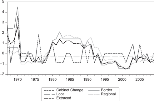
The five political instability indicators.
5 Methodology and Model
We employed two econometric techniques to compare and guarantee robust results and conclusions. These two techniques are: First, ordinary least squares (OLS): we use this method to examine the effect of political instability on real income per capita growth rate in Jordan. We estimated the following autoregressive distributed lag model (ARDL) [16]:
where
Second, Kalman filter (ML method) is an estimator useful in appraising model parameters as omission of some variables might lead to misspecification, which could result in spurious findings. This technique is the main method used here for assessing the impact of political instability on both economic growth and government expenditure. To apply Kalman filter, we outline a linear Gaussian state space model by the following measurement and state equations:
The first is a measurement equation linearly relating the observed variable
Next, we estimate the same shape of the ARDL model by employing Kalman filter. In this step, we rewrite eq. [1] to fit the state space model:
where
6 Empirical Results
The first step to extract the results by using ARDL model is to examine whether the data on the level have a unit root or not. This is an important step to avoid creating a spurious regression. Therefore, we conduct three tests: Augmented Dickey-Fuller (ADF), Phillips–Perron (PP) and Kiwathowski–Phillips–Schmidt–Shin (KPSS) unit root tests on the level with trend and intercept because the data have both. Table 4 presents the results from panel A. The three tests support non-stationary series at the levels of all the four variables. However, the KPSS results reveal that real investment and real per capita are stationary at the 1 % level. Also, we perform the three unit root tests on the first difference of the four variables with an intercept. The results reported in panel B of Table 4 show that the three tests assure a stationary series on the first difference for all the four variables. Conversely, the ADF test indicated that both money supply and real per capita have unit roots at the first differences.
The unit root tests.
| ADF | PP | KPSS | ||
|---|---|---|---|---|
| Panel A: Level form, with trend and intercept | ||||
| –2.28 (0.44) | K=2 | –1.07 (0.92) | 0.17** | |
| –1.61 (0.77) | K=1 | –0.80 (0.96) | 0.17** | |
| –2.02 (0.57) | K=0 | –2.22 (0.47) | 0.08 | |
| –2.73 (0.23) | K=2 | –2.16 (0.50) | 0.07 | |
| Panel B: First difference form, with intercept | ||||
| –1.75 (0.39) | K=1 | –2.65 (0.09)*** | 0.30 | |
| –3.89 (0.005)* | K=0 | –3.99 (0.004)* | 0.30 | |
| –6.18 (0.000)* | K=0 | –6.18 (0.000)* | 0.13 | |
| –2.41 (0.14) | K=1 | –5.77 (0.000)* | 0.12 | |
Notes: the null hypothesis of ADF and PP unit root statistics states that the series is non-stationary against the alternative hypothesis, which is stationary. At the level form, the critical values for the ADF and PP tests are –4.205, –3.526, and 3.194 at 1 %, 5 % and 10 %, respectively. The null hypothesis of the KPSS test states that the observed series is stationary versus an alternative of a unit root. The critical values for the KPSS statistics at 1 %, 5 % and 10 % are 0.216, 0.146 and 0.119, respectively. The optimal lag length k is determined based on AIC criteria (maximum lag length was 10). p-Values are reported in parentheses.*, **, and ***represent 1 %, 5 % and 10 % significance levels, respectively. At the first difference form, the critical values for the ADF and PP tests are –3.605, –2.936, and –2.606 at 1 %, 5 % and 10 %, respectively. The critical values for the KPSS statistics at 1 %, 5 % and 10 % are 0.739, 0.463 and 0.347, respectively.
Tables 5 and 6 display the estimates from the models with respect to eq. [1] and eq. [2] with eq. [3], respectively. As for determining the optimum lags of the OLS technique (eq. [1]), we use Akaike information criteria to choose the optimum number of lags [18] combined by running serial correlation. [19] Given the F-statistic critical value of 5.39 at 1% significance level, the Lagrange Multiplier (LM) test confirms autocorrelation-free residuals. In addition, we test for heteroskedasticity, since the critical F-statistic of (2.993 at 1% significance level), Harvey test cannot reject the null hypothesis of no heteroskedasticity. Further, we check for the stability of the estimated coefficients by employing Ramsey’s regression equation specification error test (RESET), and the cumulative sum of the recursive squared residuals (CUSUMQ). In the diagnostic part of Table 5, the Ramsey’s RESET test has a chi-squared distribution with a single degree of freedom. Given its critical value of 6.63 at 1% significance level, we determine that RESET statistic is smaller than the critical value for eq. [1], indicating that the model is correctly specified. Further, the latter test inspects whether the CUSUMQ goes outside the area between the two 5% critical lines or not. If it goes outside the 5% critical line, the estimated coefficients are unstable. Figure 2, in Appendix B, shows that the CUSUMQ does not cross the critical line for the five equations [20] in Table 5. We thus conclude that the estimated coefficients of the five equations are stable.
Coefficients of the eq. [1].
| Dependent variable, | |||||
|---|---|---|---|---|---|
| Constant | –0.014 (0.018) | –0.02 (0.02) | 0.001 (0.19) | 0.008 (0.02) | 0.02 (0.02) |
| 0.11 (0.17) | 0.08 (0.16) | 0.14 (0.16) | 0.11 (0.15) | 0.13 (0.15) | |
| 0.46 (0.15)*** | 0.50 (0.14)*** | 0.53 (0.14)*** | 0.55 (0.14)*** | 0.54 (0.13)*** | |
| –0.50 (0.19)*** | –0.48 (0.18)*** | –0.53 (–0.18)*** | –0.57 (0.17)*** | –0.49 (0.17)*** | |
| –0.20 (0.19) | –0.24 (0.18) | –0.22 (0.18) | –0.18 (0.17) | –0.23 (0.17) | |
| 0.27 (0.07)*** | 0.25 (0.07)*** | 0.26 (0.07)*** | 0.26 (0.06)*** | 0.23 (0.06)*** | |
| 0.04 (0.08) | 0.04 (0.07) | 0.02 (0.07) | 0.0004 (0.07) | 0.02 (0.07) | |
| –0.07 (0.14) | –0.08 (0.13) | –0.008 (0.13) | –0.08 (0.13) | –0.09 (0.12) | |
| Cabinet change ( | –01 (0.008) | – | – | – | – |
| Local instab. | – | –02 (0.006)** | – | – | – |
| Border instab. | – | – | –003 (0.001)** | – | – |
| Regional instab. | – | – | – | –001 (0.0005)*** | – |
| Total index | – | – | – | – | –05 (0.016)*** |
| Diagnostics | |||||
| 0.48 | 0.54 | 0.53 | 0.56 | 0.59 | |
| 0.87 | 1.15 | 0.05 | 0.04 | 0.02 | |
| Hetero. | 1.47 | 0.79 | 0.76 | 1.20 | 0.78 |
| RESET | 1.69 | 2.09 | 0.96 | 0.97 | 1.14 |
| CUSUMSQ | Stable | Stable | Stable | Stable | Stable |
| No. of Obs. | 41 | 41 | 41 | 41 | 41 |
Notes: Standard errors are in parentheses. */**/***denotes statistically significant at the 10/5/1 percent level, respectively.
| Dependent variable, | |||||
|---|---|---|---|---|---|
| 0.32 (0.12)*** | 0.25 (0.10)** | 0.42 (0.11)*** | 0.41 (0.11)*** | 0.43 (0.09)*** | |
| 0.19 (0.11)* | 0.27 (0.11)*** | 0.23 (0.10)** | 0.24 (0.10)** | 0.24 (0.10)*** | |
| –37 (0.18)** | –36 (0.14)*** | –39 (0.16)** | –41 (0.16)*** | –35 (0.14)** | |
| –35 (0.14)** | –0.40 (0.12)*** | –0.36 (0.13)*** | –0.33 (0.14)** | –0.37 (0.12)*** | |
| 0.23 (0.07)*** | 0.19 (0.07)*** | 0.24 (0.06)*** | 0.24 (0.05)*** | 0.22 (0.06)*** | |
| –0.05 (0.05) | –0.08 (0.05) | –0.07 (0.05) | –0.09 (0.05) | –0.07 (0.05) | |
| Cabinet change ( | –0.01 (0.007) | – | – | – | – |
| Local instab. | – | –0.02 (0.009)* | – | – | – |
| Border instab. | – | – | –0.002 (0.001)** | – | – |
| Regional instab. | – | – | – | –0.001 (0.0004)** | – |
| Total index | – | – | – | – | –0.04 (0.01)*** |
| 0.002*** | 0.002*** | 0.002*** | 0.002*** | 0.001*** | |
| 0.00003** | 0.0002*** | 0.0003*** | 0.0002*** | 0.0002*** | |
| –0.90 (0.48)* | –0.71 (0.45) | –0.72 (0.57) | –0.73 (0.56) | –0.74 (0.47) | |
| LOGL | 70.4 | 72.4 | 71.9 | 72.3 | 73.4 |
| AIC | –2.9 | –3.0 | –2.9 | –3.0 | –3.0 |
| SC | –2.5 | –2.6 | –2.5 | –2.6 | –2.6 |
| HQC | –2.7 | –2.8 | –2.8 | –2.8 | –2.9 |
| No. of Obs. | 41 | 41 | 41 | 41 | 41 |
Notes: Standard errors are in parentheses. */**/***denotes statistically significant at the 10/5/1 percent level, respectively.
The empirical results from our estimation are consistent with economic theory. Jordan’s real income per capita growth rate has a statistically significant relationship with money supply growth rate, inflation rate, and real investment growth rate with the correct signs. The growth rates of money supply and real investment have statistically significant and positive relationships with real income per capita growth rate. [21] Meanwhile, inflation rate has a statistically significant negative relationship with real income per capita growth rate. Likewise, political instability has a statistically significant negative relationship with real income per capita growth rate in Jordan. This statistically significant negative relationship is confirmed with respect to the four political instability types: local instability, border instability, regional and the total or the derived index.
The empirical findings following the application of the Kalman technique are shown in Table 6. The results are consistent with the results from OLS estimation. Obviously
7 Political Instability and Real Government Expenditures
In the previous section, we showed that political instability has a negative impact on real income per capita in Jordan. In this section, we expand the analysis by examining the relationship between political instability and real government expenditure by using the Kalman filter technique only. We believe that this extension throws light on a potential channel through which political instability affects economic growth in Jordan. On average, the share of government spending in GDP is 27 %. Usually, political instability is accompanied by a greater ambiguity about the stability of the present political regime and/or government; thus its future economic programs and policies. Hence, it is also likely to adversely affect its expenditures. In fact, most previous studies have concentrated on the relationship between political instability and investment (Özler and Rodrik 1992; and Mauro 1995) and inflation rate (Aisen and Veiga 2006; Cukierman, Edwards, and Tabellini 1992). But, none of these studies had focused on the relation between political instability and real government expenditures.
To explore the effect of political instability on real government expenditures in Jordan, we assume that expenditures are determined by the following model:
where
We estimate eqs [4] and [5] using the ML method; the results are reported in Table 7. Originally, we estimated eqs [4] and [5] with the error term but it seemed the value of the error term of eq. [4],
| Dependent variable, | |||||
|---|---|---|---|---|---|
| 1.68 (0.46)*** | 1.61 (0.03)*** | 1.65 (0.39)*** | 1.67 (0.43)*** | 1.76 (0.46)*** | |
| 0.53 (0.11)*** | 0.49 (0.19)*** | 0.67 (0.15)*** | 0.63 (0.19)*** | 0.51 (0.16)*** | |
| Constant | –1.35 (1.49) | –1.38 (1.50) | –2.32 (1.88) | –1.65 (1.44) | –1.75 (1.61) |
| Cabinet change | –0.03 (0.02)* | – | – | – | – |
| Local instab. | – | –0.07 (0.03)** | – | – | – |
| Border instab. | – | – | –0.02 (0.009)** | – | – |
| Regional instab. | – | – | – | –0.01 (0.005)** | – |
| Total Index | – | – | – | – | –0.26 (0.11)** |
| 0.030*** | 0.027*** | 0.029*** | 0.028*** | 0.026*** | |
| 0.85 (0.13)*** | 0.83 (0.14)*** | 0.75 (0.18)*** | 0.82 (0.13)*** | 0.81 (0.14)*** | |
| LOGL | 13.93 | 16.15 | 14.65 | 15.25 | 16.88 |
| AIC | –0.37 | –0.47 | –0.40 | –0.43 | –0.51 |
| SC | –0.12 | –0.23 | –0.16 | –0.19 | –0.26 |
| HQC | –0.28 | –0.38 | –0.31 | –0.34 | –0.42 |
| No. of Obs. | 41 | 41 | 41 | 41 | 41 |
Notes: Standard errors are in parentheses. */**/***denotes statistically significant at the 10/5/1 percent level, respectively.
8 Conclusions
Economists have been studying the relationship between political instability and economic growth over the last four decades. Most previous studies have demonstrated that political instability harms economic growth. Further, they showed that the transmission channel consists of disturbances in physical capital, investment, foreign direct investment, and has high inflation rate. By contrast, other studies have found a statistically insignificant link between political instability and the growth rate of real GDP per capita. Most empirical studies on the economics of political instability relied on extracting evidence from panel data of many countries. By contrast, the current paper seeks to extract evidence from a single country, Jordan.
We adopted the definition of Gyinmah–Brempong and Traynor (1999) and Burger, Ianchovichina, and Rijkers (2013) for political instability. Based on these definitions and data accessibility, we have examined political instability along four dimensions: cabinet changes in Jordan, local wars and violence, wars and violence in neighboring states, and wars and violence in regional states. Next, we extracted a fifth political instability proxy from the four proxies by using the exploratory factor analysis.
On the empirical side, we have used two techniques, OLS and Kalman filter. The findings from the current paper show that political instability has a negative effect on the growth rate of real income per capita in Jordan. Also, the current paper has concluded that political instability has a negative impact on government expenditures.
Acknowledgments
The author would like to thank the editor and two anonymous referees of Review of Middle East Economics and Finance for their valuable and helpful comments. We are responsible for any errors.
Appendix A: Data
The present paper uses five forms of political instability which they are: cabinet changes, local instability, border instability, regional instability, and total index. The definition and source of each one is as follows:
Cabinet changes: is the number of each cabinet reshuffles in each year, the source is Jordan’s prime minister website; see footnote 2.
Local instability: total major episodes of local political violence. The source is INSCR.
Border instability: total major episodes of political violence of the countries on the border. The source is INSCR.
Regional Instability: total major episodes of political violence of the countries in the region. The source is INSCR.
Total index: this index is calculated by the author from the abovementioned four forms of political instability by using principles factor analysis.
Table 8 presents all these data.
Political instability data in Jordan.
| Cabinet change | Local instability | Boarder instability | Regional instability | Total index | |
|---|---|---|---|---|---|
| 1967 | 4 | 4 | 15 | 30 | 1.66 |
| 1968 | 0 | 4 | 15 | 30 | 1.29 |
| 1969 | 2 | 4 | 15 | 28 | 1.46 |
| 1970 | 5 | 7 | 15 | 31 | 2.04 |
| 1971 | 1 | 0 | 7 | 13 | 0.52 |
| 1972 | 1 | 0 | 7 | 13 | 0.52 |
| 1973 | 1 | 0 | 13 | 17 | 0.83 |
| 1974 | 1 | 0 | 8 | 14 | 0.57 |
| 1975 | 0 | 0 | 8 | 17 | 0.50 |
| 1976 | 3 | 0 | 7 | 15 | 0.72 |
| 1977 | 0 | 0 | 7 | 16 | 0.45 |
| 1978 | 0 | 0 | 9 | 27 | 0.63 |
| 1979 | 1 | 0 | 13 | 31 | 0.94 |
| 1980 | 2 | 0 | 19 | 41 | 1.39 |
| 1981 | 0 | 0 | 20 | 40 | 1.24 |
| 1982 | 0 | 0 | 24 | 48 | 1.49 |
| 1983 | 0 | 0 | 20 | 50 | 1.31 |
| 1984 | 1 | 0 | 20 | 53 | 1.43 |
| 1985 | 1 | 0 | 20 | 53 | 1.43 |
| 1986 | 0 | 0 | 20 | 50 | 1.31 |
| 1987 | 0 | 0 | 20 | 50 | 1.31 |
| 1988 | 0 | 0 | 20 | 48 | 1.30 |
| 1989 | 2 | 0 | 14 | 36 | 1.11 |
| 1990 | 0 | 0 | 19 | 46 | 1.24 |
| 1991 | 2 | 0 | 15 | 50 | 1.26 |
| 1992 | 0 | 0 | 10 | 36 | 0.74 |
| 1993 | 1 | 0 | 10 | 36 | 0.83 |
| 1994 | 0 | 0 | 5 | 25 | 0.42 |
| 1995 | 1 | 0 | 5 | 18 | 0.46 |
| 1996 | 1 | 0 | 6 | 19 | 0.52 |
| 1997 | 1 | 0 | 6 | 19 | 0.52 |
| 1998 | 1 | 0 | 7 | 18 | 0.56 |
| 1999 | 1 | 0 | 3 | 13 | 0.33 |
| 2000 | 1 | 0 | 3 | 9 | 0.30 |
| 2001 | 0 | 0 | 3 | 9 | 0.21 |
| 2002 | 1 | 0 | 3 | 9 | 0.30 |
| 2003 | 2 | 0 | 9 | 14 | 0.71 |
| 2004 | 0 | 0 | 9 | 16 | 0.54 |
| 2005 | 2 | 0 | 9 | 16 | 0.73 |
| 2006 | 0 | 0 | 11 | 20 | 0.67 |
| 2007 | 1 | 0 | 9 | 17 | 0.64 |
| 2008 | 0 | 0 | 8 | 17 | 0.50 |
| 2009 | 1 | 0 | 8 | 15 | 0.58 |
Appendix B: Plot of Cumulative Sum of the Recursive Squared Residuals
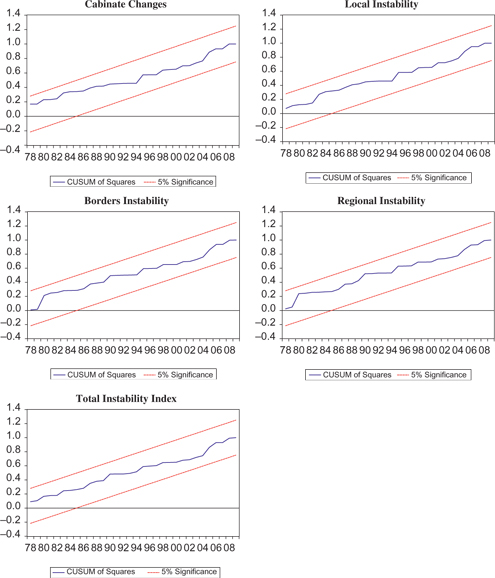
Plot of cumulative sum of the recursive squared residuals (CUSUMQ) for growth rate of real income per capita.
References
Aisen, A., and F. J. Veiga. 2006. “Does Political Instability Lead to Higher Inflation? a Panel Data Analysis”. Journal of Money, Credit and Banking 38 (5):1379–89.10.1353/mcb.2006.0064Search in Google Scholar
Aisen, A., and F. J. Veiga. 2013. “How Does Political Instability Affect Economic Growth?” European Journal of Political Economy 29 (March):151–67.10.1016/j.ejpoleco.2012.11.001Search in Google Scholar
Alesina, A., S. Ozler, N. Roubini, and P. Swagel. 1996. “Political Instability and Economic Growth”. Journal of Economic Growth 1 (2):189–211.10.3386/w4173Search in Google Scholar
Alesina, A., and R. Perotti. 1996. “Income Distribution, Political Instability, and Investment”. European Economic Review 40 (6):1203–28.10.3386/w4486Search in Google Scholar
Alfaro, L., S. Kalemli-Ozcan, and V. Volosovych. 2008. “Why Doesn’t Capital Flow From Rich to Poor Countries? An Empirical Investigation.” Review of Economics and Statistics 90 (2):347–68.10.3386/w11901Search in Google Scholar
Barro, R. 1991. “A Cross Country Study of Growth, Saving and Government.” In National Saving and Economic Performance, edited by S. Bernheim. Cambridge, MA: NBER.Search in Google Scholar
Burger, M., E. Ianchovichina, and B. Rijkers. 2013. “Political Instability and Greenfield Foreign Direct Investment in the Arab World.” The World Bank, Middle East and North Africa Region, Policy Research Working Paper 6716, December.10.1596/1813-9450-6716Search in Google Scholar
Busse, M., and C. Hefeker. 2007. “Political Risk, Institutions and Foreign Direct Investment”. European Journal of Political Economy 23 (2):397–416.10.1016/j.ejpoleco.2006.02.003Search in Google Scholar
Campos, N., and J. Nugent. 2002. “Who Is Afraid of Political Instability”. Journal of Development Economics 62 (1):157–72.10.1016/S0304-3878(01)00181-XSearch in Google Scholar
Campos, N., J. Nugent, and J. A. Robinson. 1999. “Can Political Instability Be Good for Growth? The Case of The Middle East and North Africa.” Department of Economics, University of Southern California, January.Search in Google Scholar
Choucair, J. 2006. “Illusive Reform: Jordan’s Stubborn Stability.” Carnegie Endowment for International Peace, Carnegie paper, No. 76, December.Search in Google Scholar
Collier, P. 1999. “On the Economic Consequences of Civil War”. Oxford Economic Papers 51 (1):168–83.10.1093/oep/51.1.168Search in Google Scholar
Cukierman, A., S. Edwards, and G. Tabellini. 1992. “Seigniorage and Political Instability”. American Economic Review 82 (3):537–55.10.3386/w3199Search in Google Scholar
Daude, C., and E. Stein. 2007. “The Quality of Institutions and Foreign Direct Investment”. Economics and Politics 19 (3):317–44.10.1111/j.1468-0343.2007.00318.xSearch in Google Scholar
De Haan, J., and C. Siermann. 1996. “Political Instability, Freedom, and Economic Growth: Some Further Evidence”. Economic Development and Cultural Change 44 (2):339–50.10.1086/452217Search in Google Scholar
Gupta, D. 1990. The Economics of Political Violence: The Effect of Political Instability on Economic Growth. New York: Praeger Publishers.Search in Google Scholar
Gyimah-Brempong, K., and T. L. Traynor. 1999. “Political Instability, Investment and Economic Growth in Sub-Saharan Africa”. Journal of African Economies 8 (1):52–86.10.1093/jae/8.1.52Search in Google Scholar
Hamilton, J. 1994. Time Series Analysis. Princeton, NJ: Princeton University Press.10.1515/9780691218632Search in Google Scholar
Harrigan, J., W. Chengang, and H. El-Said. 2006. “The Economic and Political Determinants of IMF and World Bank Lending in the Middle East and North Africa”. World Development 34 (2):247–70.10.1057/9781137001597_2Search in Google Scholar
Harrigan, J., and C. Wang. 2004. “A New Approach to Aid Allocation Among Developing Countries: Is The US More Selfish Than the Rest?” School of Economic Studies Working Paper Series No. 04/11. University of Manchester.Search in Google Scholar
Hahs-Vaughn, D., and R. Lomax. 2013. An Introduction to Statistical Concepts, 3rd edn. New York: Routledge.10.4324/9780203137819Search in Google Scholar
Harvey, A. C. 1989. Forecasting, Structural Time Series Models and the Kalman Filter. Cambridge: Cambridge University Press.10.1017/CBO9781107049994Search in Google Scholar
Jong-A-Pin, R. 2009. “On the Measurement of Political Instability and Its Impact on Economic Growth”. European Journal of Political Economy 25 (1):15–29.10.1016/j.ejpoleco.2008.09.010Search in Google Scholar
Kirmanoglu, H. 2003. “Political Freedom and Economic Well-Being: A Causality Analysis.” International Conference on Policy Modeling, Istanbul, Turkey.Search in Google Scholar
Maddala, G. S., and I.-M. Kim. 1998. Unit Roots Cointegration, and Structural Change. Cambridge: Cambridge University Press.10.1017/CBO9780511751974Search in Google Scholar
Maizels, A., and M. K. Nissanke. 1984. “Motivations for Aid to Developing Countries”. World Development 12 (9):879–900.10.1016/0305-750X(84)90046-9Search in Google Scholar
Mauro, P. 1995. “Corruption and Growth”. Quarterly Journal of Economics 110 (3):681–712.10.2307/2946696Search in Google Scholar
Olson, M. 1991. “Autocracy, Democracy, and Prosperity.” In Richard Zeckhauser, ed., Strategy and Choice.Search in Google Scholar
Ozler, S., and D. Rodrik. 1992. “External Shocks, Politics and Private Investment: Some Theory and Empirical Evidence”. Journal of Development Economics 39 (1):141–62.10.3386/w3960Search in Google Scholar
Ramachandran, S. 2004. Jordan Economic Development in the 1990s and World Bank Assistance. Washington, D.C.: The World Bank.Search in Google Scholar
Rodrik, D. 1989. “Policy Uncertainty and Private Investment in Developing Countries”. NBER Working Paper No. 2999.10.3386/w2999Search in Google Scholar
Rodrik, D. 1995. “Why is There Multilateral Lending”. NBER Working Paper (June) No. W5160.10.3386/w5160Search in Google Scholar
Schneider, F., and B. S. Frey. 1985. “Economic and Political Determinants of Foreign Direct Investment”. World Development 13 (2):161–75.10.1016/0305-750X(85)90002-6Search in Google Scholar
Sharp, J. M. 2014. “Jordan: Background and U.S. Relations, Congressional Research Service.” January. Available at: http://www.fas.org/sgp/crs/mideast/RL33546.pdf.Search in Google Scholar
Sweidan, O. 2013. “Exchange Rate Pass-Through Into Import Prices in Jordan”. Global Economy Journal 13 (1):109–28.10.1515/gej-2012-0013Search in Google Scholar
United Nation. 2015. “World Economic Situation and Prospects: Chapter One, Global Economic Outlook.” Available at: http://www.un.org/en/development/desa/policy/wesp/wesp_archive/2015wesp_chap1.pdf10.18356/037deb21-enSearch in Google Scholar
Wansbeek, T., and E. Meijer. 2000. Measurement Error and Latent Variables in Econometrics. Amsterdam: North Holland.Search in Google Scholar
Worman, J. G., and D. H. Gray. 2012. “Terrorism in Jordan: Politics and the Real Target Audience”. Global Security Studies 3 (3):94–112.Search in Google Scholar
Zablotsky, E. 1996. “Political Stability and Economic Growth.” CEMA Working Papers 109, Universidad del CEMA.Search in Google Scholar
Zeaiter, H., R. El-Khalil, and K. Fakih. 2015. “Economic Development and Sub-Regional Identities” The Journal of Developing Areas 49 (1):157–76.10.1353/jda.2015.0032Search in Google Scholar
Zureiqat, H. M. 2005. “Political Instability and Economic Performance: A Panel Data Analysis.” http://digitalcommons.macalester.edu/econaward/1.Search in Google Scholar
©2016 by De Gruyter
Articles in the same Issue
- Frontmatter
- Spatial Propagation of the Economic Impacts of Bombing: The Case of the 2006 War in Lebanon
- Designing a Fiscal Framework for a Prospective Commodity-producer: Options for Lebanon
- Political Instability and Economic Growth: Evidence from Jordan
- Food and Agricultural Trade in the GCC: An Opportunity for South Asia?