Slavery versus Labor
-
Giuseppe Dari-Mattiacci


Abstract
Slavery has been a long-lasting and often endemic problem across time and space, and has commonly coexisted with a free-labor market. To understand (and possibly eradicate) slavery, one needs to unpack its relationship with free labor. Under what conditions would a principal choose to buy a slave rather than to hire a free worker? First, slaves cannot leave at will, which reduces turnover costs; second, slaves can be subjected to physical punishments, which reduces enforcement costs. In complex tasks, relation-specific investments are responsible for high turnover costs, which makes principals prefer slaves over workers. At the other end of the spectrum, in simple tasks, the threat of physical punishment is a relatively cheap way to produce incentives as compared to rewards, because effort is easy to monitor, which again makes slaves the cheaper alternative. The resulting equilibrium price in the market for slaves affects demand in the labor market and induces principals to hire workers for tasks of intermediate complexity. The available historical evidence is consistent with this pattern. Our analysis sheds light on cross-society differences in the use of slaves, on diachronic trends, and on the effects of current anti-slavery policies.
1 Introduction
Every human society has experienced slavery at some point in the course of its history, mostly under the cover of legality. Some of the most famous US presidents owned slaves.[1] Although Article 4 of the Universal Declaration on Human Rights (1948) proclaims that “no one should be held in slavery or servitude, slavery in all of its forms should be eliminated,” according to the International Labor Organization, “at any given time in 2016, an estimated 40.3 million people are in modern slavery, including 24.9 million in forced labour and 15.4 million in forced marriage.”[2] The problem is not confined to countries with low regard for human rights; in 2017, the New York Times published an article entitled “Slavery Ensnares Thousands in U.K.”[3] While exact numbers are very difficult to pin down, there is widespread recognition that slavery is a global problem affecting, in some cases, large portions of the local population and generating billions of dollars in illegal profits.[4]
So far the scholarly discussion has largely focused on slaves alone, providing limited insights into the interplay between slavery and free labor. In truth, slaves and free workers have regularly competed for the same jobs in all slave societies and continue to do so today. Changes in the labor market are bound to affect the slave market and vice versa. Improving our knowledge of the dynamics of slavery requires understanding the drivers of an employer’s choice between slavery and labor, its implications for the (free and forced) labor market, and its effects on the workers’ behavior and well-being. This paper provides the first integrated model of slavery and labor, examines the available historical evidence through the lens of the model’s findings, and draws implications for current anti-slavery policies. In particular, given a dual-status regime where some individuals are “slaves” while others are “free workers” and a market for each of them, we seek to answer the question whether employers will hire free workers or buy slaves for different types of occupations.[5] Figure 1 illuminates the empirical fact that inspires our model: across history, slaves tended to be employed more often in either complex or simple tasks, leaving tasks of intermediate complexity mainly for free workers (details are provided in Section 6.2).

Prevalence of slavery along the task complexity continuum. Each line refers to a different macro region of the Empire of Brazil (1822–1889), as characterized by the level of turnover costs (β) and abundance of slaves (γ). Source: The Brazilian Census of 1872.
We begin from the observation that slaves are fundamentally different from free workers along two key dimensions: the participation dimension and the incentive dimension. First, while workers can exit at will, slaves cannot, and hence the employer may bear turnover costs only if she hires a worker. In fact, this somewhat extreme perspective captures a more nuanced reality. Although also the freedom of workers can be limited in various ways, it is easier for employers to retain a slave than to retain a free worker. Second, slaves can be subjected to physical punishments (sticks) in addition to rewards (carrots), which are the only incentive available for workers. As above, although also free workers can be subjected to a diverse array of punishments, our approach captures in a simple way the fact that punishments are more commonly condoned if applied to slaves than to free workers. Employers factor in these two “advantages” of slaves over workers when choosing between the two.
In the model, a principal employs an agent – that is, hires a free worker or buys a slave – to execute a task. Free workers and slaves are identical but for the two differences highlighted above. The complexity of the task is a key component of the analysis. In complex tasks, relation-specific investments are responsible for high turnover costs, which makes employers prefer slaves over workers. At the other end of the spectrum, in simple tasks, the threat of physical punishment is a relatively cheap way to produce incentives as compared to rewards because effort is easy to monitor, which again makes slaves the better alternative. Consequently, principals are willing to pay more for a slave in complex and simple tasks than in tasks of intermediate complexity, where both monitoring and labor turnover are only mildly problematic. The resulting equilibrium price in the market for slaves affects demand in the labor market and induces principals to hire workers for those intermediate tasks.
The aforementioned equilibrium depends on the level of turnover costs, the cost of sticks, and the abundance of slaves. Our theory provides comparative statics for the distribution of tasks between slaves and workers, their respective prevalence as agents, and the proportion of slaves in complex tasks relative to slaves in simple tasks. First, if turnover costs increase, if sticks become cheaper, or if the supply of slaves increases, then slaves will be employed more frequently overall and, consequently, workers will be employed less frequently. Second, an increase in the cost of sticks changes the mix of tasks assigned to slaves, raising the slaves’ welfare. An increase in turnover costs and an increase in slave supply raise slaves’ welfare only if there are enough slaves performing simple tasks.
A critical postulate distinguishes our approach from others. We start from the observation that, throughout history, slavery has been largely a matter of status, defined and enforced by state power. From a principal’s perspective, the population is divided into two groups: the free (who can be hired) and slaves (who can be purchased). Whether an individual falls into one or the other category is a matter of law and individual history (as in Lagerlöf 2016), rather than the principal’s decision (as in Domar 1970; Acemoglu and Wolitzsky 2011).[6] Therefore, the focus of our model is not the question of whether the principal will invest resources to coerce an agent. To the contrary, we take an agent’s status as a given, and reduce the principal’s choice to a decision between hiring a worker and buying a slave. In turn, this perspective allows us to study the use of workers and slaves as alternative means of production in slave systems that are (more or less actively) sponsored by the state or on which the state turns a blind eye.[7]
Our historical analysis focuses mainly on Ancient Rome and the Americas during the period of European colonization, with occasional references to other episodes. These two historical periods are unmatched in terms of the size of their slave populations and the reliance of their economies on slavery. We zero in on cases in which we could find occupational data on both the slave and the free population, and first review the available evidence qualitatively. We then study the unique Brazilian Census of 1872, which is, to our knowledge, the only dataset that records the distribution of occupations among slaves and free workers. The lack of detailed data makes it hard to find exogenous variations in our model’s parameters. We hence resort to three complementary strategies to elicit variation indirectly: we compare regions that exhibited clearly different values in one of our parameters of interest; we infer variation in one of the parameters from geography; and, finally, we exploit exogenous changes in the supply of slaves, such as wars. Although we come nowhere close to a satisfactory causal identification and the reader may disagree with our classification of tasks, with these caveats in mind, both the qualitative and the quantitative evidence are consistent with our model’s predictions (as previewed in Figure 1).
Finally, this article offers some cautious insights on the ongoing struggle against forced labor. According to Beate Andrees of the International Labor Organization, “ending bonded labor will require economic as well as legal measures.”[8] Such measures are usually targeted towards cutting the slave supply, which reduces the prevalence of slavery. We warn, however, about possible inframarginal effects on the conditions in which remaining slaves will live. Only an increase in the cost of sticks unambiguously moves slaves from tasks mostly enforced by sticks to tasks mostly enforced by carrots. Legal reforms solely aimed at reducing turnover costs or hindering the slave supply might worsen the living conditions of the remaining slaves by pushing them towards tasks largely enforced by sticks.
This article is organized as follows: Section 2 frames our paper in the current literature; Section 3 discusses our theory; Section 4 analyzes the comparative statics of our model; Section 5 relaxes some of the key assumptions of our theory; Section 6 tests the results of our model against available evidence; Section 7 debates the main issues of past and current abolition strategies; Section 8 offers a summary of our results and ideas for future research.
2 Scope of the Analysis and Relation to the Literature
In this section, we emphasize the two assumptions defining the scope of our analysis – slave status and the integrated market for slaves and workers – and dissect the explanations given in the extant literature for the choice between buying a slave and hiring a worker.
2.1 Slave Status
State coercion and a system of laws clearly defining slave status are crucial to maintaining a slave population (Baptist 2014, p. 64; Coclanis 2010, pp. 490, 500; Davies 2007, p. 352; Morris 1999, p. 9; Peabody 2011, p. 598; Scarano 2010, p. 35; Wright 2006, p. 12). The Roman jurist Gaius epitomized this point: “[T]he great divide in the law of persons is this: all men are either free men or slaves.” (Digest 1.5.3).[9] Roman law further specified the conditions under which a person could be considered a slave, which was viewed as a legal construct “against nature” (Digest 1.5.4.1 and 1.5.5). Capture in war and birth from a female slave were the most common reasons (Gardner 2011, p. 415; Scheidel 2011, p. 296; Temin 2013, p. 121). This partition was of crucial importance and was meticulously enforced. Most importantly, slaves were considered things that could be bought and sold; harm to a slave was viewed as property damage, just like harm to cattle (Digest 1.5.4.1 and 9.2.2 pr.).
European colonies in the Americas quickly created laws to distinguish African slaves from free or indentured European workers and Native American laborers (Forret 2010, p. 277; Littlefield 2010, p. 203; Peabody 2011, p. 600; Tomlin (2010, p. 402); Wright 2006, p. 6). Legislation was essential in order to keep “slaves as outsiders, rootless and ahistorical individuals [who were] ultimately held against their will by the threat of force” (Klein and Vinson 2007, p. 30). For instance, a 1712 South Carolina statute read: “All negros, mulattoes, mestizo’s or Indians, which at any time heretofore have been sold, or now are held or taken to be, or hereafter shall be bought and sold for slaves, are hereby declared slaves; and they, and their children, are hereby made and declared slaves” (Morris 1999, p. 46). For employers, such state-sponsored slave systems meant that they could “either use Europeans hired on contract as indentured servants; or use Africans, captured and enslaved” (Littlefield 2010, p. 281).
Accordingly, in the model we take an agent’s status as exogenously given: a principal cannot coerce a free agent into slavery but can purchase an agent with slave status (as in Lagerlöf 2016).[10] In contrast, two very influential contributions in the literature, Domar (1970) and Acemoglu and Wolitzsky (2011), focus on the investment in coercion, thereby endogenizing slave status. These models have different domains of application. While theirs can be used to explain coercion between individuals or groups – such as human trafficking by criminal organizations or the emergence of serfdom in Eastern Europe – our model is tailored towards state-sponsored slavery.
2.2 Integrated Slave and Labor Markets
There is ample historical evidence that slaves and workers supplied labor in an integrated market, where principals could choose between them and often employed both. It is therefore unsatisfactory to study the slave market and the (free) labor market in isolation. Slave prices and workers’ wages were critically related, with supply in one market affecting prices in the other and vice versa. Scheidel (2008, pp. 106, 115) and Temin (2013, pp. 115, 134) have made this point forcefully in the context of the Roman economy. The situation was similar in the Americas and in other slave societies (Klein and Vinson 2007, pp. 17, 29). Forret (2010, p. 276) notes that “[t]ransitions to African slavery in the several colonies of England’s emerging empire can be better understood if Britain’s Atlantic world is approached as a single if imperfect and fragile labor market and if variations in the composition of the workforce among colonies and within particular colonial regions over time are approached through a focus on the supply and demand for labor”. Accordingly, “market prices would adjust to place some employers at the margin of choice between the different types of labor” (Hanes 1996, p. 313).
In both historical episodes, the evidence indicates that slaves and workers were competing inputs across a variety of tasks (Davies 2007, p. 347; Forret 2010, p. 276; Hanes, 1996; Klein and Vinson 2007, p. 3; Rediker 2008, p. 269; Walsh 2011, p. 423; Weidemann 1981, p. 2). Table 1 illustrates the range of tasks to which slaves were assigned across history. Competition, however, does not imply interchangeability. As our analysis shows, inframarginal principals were not indifferent between buying a slave and hiring a worker. To the contrary, they preferred slaves to workers and vice versa depending on the characteristics of the task assigned and the prevalent prices in both markets. We will demonstrate that preference for slaves in certain tasks and for workers in others emerges in equilibrium in a predictable way.
Examples of complex and simple tasks executed by slaves across history discussed in Section 6.
| Activity | Example of tasks |
|---|---|
| Liberal jobs | Surgeon, musician, healer, hospital worker, manager, |
| tooth puller. | |
| Military | Soldier, army officer |
| Maritime and fishing | Commander, navigator, sailor, sail maker, shipbuilder |
| Industrial and commercial top jobs | Bookkeeper, business agent. |
| Industrial workers | Industry worker, spinner, miller, tanner, metalworker, |
| powder works, brick maker, indigo maker, carpenter, | |
| blacksmith, wheel maker, cabinet maker, shoemaker, | |
| goldsmith, cooper, rum maker, woodsman, silversmith, | |
| mason, seamstress, cigar maker, basket maker, leather | |
| worker, cart maker, can writer, baker, potter, carver, | |
| painter/plasterer, tinner, hat maker, mattress-maker, | |
| fine China maker. | |
| Agricultural workers | Farm manager, cowboy, sugar refiner, herdsman, |
| foremen, driver, cotton press operator, lumberjack, levee | |
| worker, plowman, horse groomer, axeman, sugar worker. | |
| Wage workers | Barber, hunter, sawyer, innkeeper, roofer, chaser of |
| runaway slaves, tailor, vegetable vendor, milk vendor, | |
| butcher, street vendor, tool sharpener, rower, caulker, | |
| jockey, gravedigger, miner, daily worker, laborer. | |
| Domestic service | Domestic servant, cook, confectioner, interpreter, child |
| care, wetnurse, watchman, midwife, executioner, launder, | |
| cart driver, coach driver, nurse, gardener. |
-
Brazilian Census of 1872; Fenoaltea (1984); Fogel (1989); Aubert (1994); Higman (1995); Hanes (1996); Wright (2006); Davies (2007); Frier and Kehoe (2007); Gardner (2011); Harris (2007); Kehoe (2007); Klein and Vinson (2007); Blanchard (2010); Burnard (2010); Childs and Barcia (2010); den Heijer (2010); Lohse (2010); Morgan (2011); Fragoso and Rios (2011); Morley (2011); Phillips (2011); Walsh (2011); Temin (2013); Dari-Mattiacci (2013); Gamauf (2016). We have listed a task if at least one of the sources mentions that that task was performed by slaves. The classification is our own elaboration of the information provided in the sources.
2.3 Competing Explanations for the Choice Between Slaves and Workers
The literature offers three main theories of the allocation of tasks between slaves and workers, based on the distinction between effort-intensive and care-intensive activities, turnover costs, and the labor-land availability ratio.
2.3.1 Effort-Intensive versus Care-Intensive Activities
In a ground-breaking paper, Fenoaltea (1984) views slave tasks along a continuum from effort-intensive activities, such as mining or gang labor in plantations, to care-intensive activities, such as crafts or business agency. Pain incentives are adequate for effort-intensive activities but are not well suited for care-intensive activities because pain-induced motivation creates anxiety and makes workers careless. Therefore, as we move from effort-intensive to care-intensive activities, we should observe that rewards, such as the prospect of manumission, become more common. Manumission, however, gives the slave control over his participation constraint, which in turn makes a slave more similar to a worker. Therefore, more slaves than workers should be found in effort-intensive activities, and vice versa in care-intensive activities. This result finds support in the study of slavery in the Antebellum United States by Fogel and Engermann (1974).
However, the distinction between effort-intensive and care-intensive activities and the prevalence, respectively, of pain and reward incentives runs against some contradictory evidence in other contexts. Tobacco production in the United States and Cuba was a care-intensive activity not necessarily dominated by workers; similarly to the cereal and vine industries (Barcia and Childs 2010, p. 94; Scheidel 2008, p. 108; Wright 2006, p. 81). Slaves did not necessarily work in the gangs found in the prototypical effort-intensive cultures. In contrast, “[M]any farmers chose to use only a few slaves, often just one or two. On small farms, a slave worked alongside family members, performing similar tasks in similar ways.” (Hanes 1996, p. 309). Moreover, slaves dominated care-intensive activities such as herding and domestic service in antiquity, despite high rates of manumission (Klein and Vinson 2007, p. 25).
Also, in antiquity there was a proliferation of free rowers in Greece and Rome, and free miners in Roman Spain, Dacia, and Egypt, both very unpleasant and dangerous activities (Scheidel 2008, p. 111). Even in mining, slaves were not necessarily the default unskilled source of labor: in Peru, black slaves supervised native labor (Blanchard 2010, p. 72). We move away from the distinction between effort and care and focus on the informational characteristics of tasks. Our perspective gives less consideration to the agent’s behavioral reactions to incentives, which was at the core of Fenoaltea’s (1984) approach, instead putting more weight on the limitations of the principal’s ability to observe effort (as in Dari-Mattiacci 2013).
2.3.2 Turnover Costs
Hanes (1996), in a study on slavery in British America, views slaves as means to decrease turnover costs.[11] Whenever a worker quits, an employer must search for and train a new worker.[12] Especially in farming, labor disruptions also decrease production because crucial tasks – such as harvesting – are not executed in due time. Since turnover costs decrease with the thickness of local labor markets, the impossibility for slaves to leave at will is especially valuable in thin local labor markets. However, this theory does not handle well instances such as the extensive use of slave labor in Baltimore (Whitman 1997, p. 6–8) and in urban areas across Brazil (Fragoso and Rios 2011, p. 351), which had relatively thick markets. There is also evidence that turnover costs were not a problem for many industries that nevertheless employed slaves (Scheidel 2008, p. 112). A final but important shortcoming of looking at turnover costs alone is that it is difficult to disentangle the exogenous and endogenous components of turnover costs. For instance, population density determines the thickness of the local labor market. Yet, population density depends on exogenous factors such as climate, and on endogenous factors such as the location of industrial clusters. Our approach combines consideration for turnover costs with an analysis of the informational characteristics of the principal–agent relationship between employer and worker.
2.3.3 Labor-Land Availability Ratio
In order to explain differences in African and Asian slave societies, Watson (1980) introduces an “openness” continuum, where openness is a function of the probability of manumission and the social status of freedmen. African societies were open societies because manumission was frequent and slaves were usually integrated into their owners’ families. Conversely, Asian societies made manumission extremely difficult due to social stigma. Similarly to Domar (1970), Lagerlöf (2009) and Acemoglu and Wolitzky (2011), Watson (1980, p. 10) explains these differences as a function of the labor-land availability ratio: labor scarcity was the key issue in Africa, whereas lack of land was the central problem in Asia. Therefore, it was natural for Africans to prioritize labor over land. Other authors, such as Scheidel (2008), have applied this framework to rank different societies: Africa and Rome were open societies; Ancient Greece and Brazil were somewhere in the middle of the continuum; the Antebellum US and the Caribbean were closed societies. But it is not clear whether openness of the slave systems affected the allocation of tasks between slaves and workers, or the other way around. In fact, it could well be that it is the use of carrots in general and of manumission in particular that made a particular system more or less open (Dari-Mattiacci, 2013). While endogenizing openness, in the model, we also vary the relative supply of slave labor.
3 Theoretical Framework
3.1 Setup
In the model, we build on Dari-Mattiacci (2013) by adding consideration for the labor market and its interaction with the slave market. A principal employs an agent to perform a task q (the principal’s type), where q is uniformly distributed on
Imperfect monitoring.
| e = 0 | e = 1 | |
|---|---|---|
| r = 1 | 1 − q | q |
| r = 0 | q | 1 − q |
Agents are of two types: slaves and free workers, which differ along two dimensions: (i) while workers may decide to leave (thereby imposing a turnover cost τ > 0 on the principal in expectation), slaves do not have this option (τ = 0); (ii) slaves can be subjected to physical punishments (sticks) in addition to rewards (carrots), while workers can only be incentivized with carrots.[15] Agents are otherwise homogeneous; in particular, slaves and workers are equally productive,[16] do not have a priori characteristics that make them more fit for a particular task,[17] and receive the same on-the-job training. Finally, both the principal and the agent are risk neutral.[18] This allows us to isolate the problem of interest from other considerations.
The parties’ payoffs are as follows:
If the agent exerts effort, he earns the carrot c with probability q, faces the stick s with probability 1 − q, and bears the cost of effort e = 1. If instead the agent does not exert effort, he earns a carrot (by mistake) with probability 1 − q and pays correctly a stick s with probability q. The principal earns v if the agent exerts effort (and zero otherwise), and pays costs τ (the turnover costs if the agent leaves before completing the task), η (the enforcement costs borne to incentivize the agent), and ζ (the purchase price of the slave or the wage of the worker), all of which will be specified below and will depend on the complexity of the task q and the type of agent (slave or worker). We initially assume that v is large enough, so that ΠP > 0, in order to focus on the choice between slaves and workers, rather than the demand for labor. (We account for the residual case in Section 5.2.)[19]
The relationship between the principal and the agent unfolds over five dates:
Date 0 (slavery v. labor): The principal either buys a slave or hires a worker.[20]
Date 1 (carrots v. sticks): The principal determines the magnitude of the carrot (for workers and slaves) and the stick (for slaves only).
Date 2 (turnover and effort): Agents learn on the job. Then the worker might leave, imposing turnover costs on the principal. (Slaves cannot leave). The agent or his replacement decides whether to exert effort.
Date 3 (monitoring and enforcement): The principal applies the stick or the carrot after observing the signal r.
Date 4 (payoffs): Payoffs of realized.
We describe and solve the model backwards, starting from date 2; actions at date 3 are mechanical.
3.2 Turnover and Effort
Turnover is not equally costly in all tasks; rather, it decreases in q. Simple tasks (high q) carry with them low turnover costs because they require little on-the-job training. Instead, in complex tasks (low q) that require investment in firm-specific knowledge, turnover may be very costly.[21] We assume the following simple functional form for the turnover costs of workers (they are 0 for slaves):
where β > 0 is a parameter capturing both the dependence of turnover costs on complexity and the (exogenous) probability that a worker will leave. (If the worker leaves, his replacement faces the same incentives to exert effort.) Both slaves and workers choose whether to exert effort. Comparing the agent’s payoffs in (3.1), the agent weakly prefers to exert effort, e = 1, if:
This is the incentive-compatibility constraint; due to risk neutrality, carrots and sticks are perfect substitutes. As it is well-known, enforcement errors (low q) dilute incentives and require larger rewards or punishments. As is easy to verify, due to the monotonicity of the costs of carrots and sticks introduced below, it is suboptimal to use a mix of both carrots and sticks. Hence, in the following we focus on the principal’s choice between a carrot
3.3 Carrots versus Sticks
The principal chooses between carrots and sticks depending on which enforcement mode yields the lower cost, η. Giving a reward c to the agent costs the principal the same amount
In contrast, imposing a punishment s costs the principal ks, where k > 0 captures the different costs that carrots and sticks may impose on the principal: with k < 1 a carrot costs more than a stick, and vice versa with k > 1. This setup fits well – but not exclusively – scenarios where carrots are monetary rewards – and hence cost what they are worth – and sticks are physical punishments – and hence may cost more or less than the pain they impose; for instance, the costs of applying a physical punishment for the principal may include (temporary) losses of productivity.[23] Given that a stick is applied with probability 1 − q to complying agents, the expected cost of sticks is:
The principal chooses carrots if η c < η s and sticks otherwise.[24] Let q* be the level of q that leaves the principal indifferent between carrots and sticks (η c = η s ):
In complex tasks,

Carrots versus sticks along the task-complexity continuum.
The principal can only apply sticks to slaves, not workers. Therefore, buying a slave reduces enforcement costs for simple tasks, q > q*, while it has no effect on the cost of enforcement in complex tasks, where both workers and slaves are incentivized through carrots. Since q* is monotonically increasing in k, the low-q region in which carrots are preferred over sticks expands as sticks become relatively more expensive – that is, as k increases. Figure 3 displays the payoff of slaves and workers as a function of the principal’s choice between carrots and sticks, and points to a dramatic discontinuity at the point where the principal switches from carrots to sticks. A decrease in q – that is, greater complexity – increases the agent’s payoff from carrots because greater information rents are paid when monitoring is more noisy. For the same reason, the expected disutility from sticks decreases as q increases because enforcement noise is tackled by greater sticks. The figure also shows that if the principal uses sticks, the slave has a negative payoff and – quite obviously – participates only because he cannot do otherwise.

Agents’ payoff along the task-complexity continuum.
3.4 Slavery versus Labor
The principal is a price-taker both on the labor market and on the market for slaves. Individual principals’ decisions are aggregated to determine demand in these markets. In the equilibrium, a principal buys slaves and uses carrots for low values of q, hires workers for intermediate values of q, and buys slaves but uses sticks for high values of q. The proof of this result (formally stated in Proposition 1 below) requires finding two values of q that leave the principal indifferent between slaves and workers, which will be denoted as
3.4.1 The Choice of a Price-Taking Principal Between Slavery and Labor
The principal maximizes her payoff subject to the subgame choices described above. Since v is a constant, we can focus on the minimization of the sum of turnover, enforcement and employment costs ζ + η + τ, where
We make here an important assumption: worker wages and slave prices do not depend on q and hence can be taken as fixed for the population of price-taking principals. This assumption reflects our setup, in which the pool of slaves and workers is homogenous with respect to qualifications and abilities and differs only at a later stage due to on-the-job training (which is the source of turnover costs). Although this is clearly a simplifying assumption – because prices are sensitive to individual abilities and the latter vary greatly – it allows us to zero in on the choice between a slave and a worker given the same abilities or varying but unobservable abilities. Allowing abilities to vary in an observable way would make both the worker wage and the slave price vary accordingly, possibly leaving their difference unchanged.
In addition, we assume that the worker’s outside option at date 0 is 0 and hence we set w = 0. We can then interpret p as the premium that the principal pays for buying a slave rather than hiring a worker. Paying the slave premium only makes sense if p does not exceed the sum of the savings in turnover costs, τ, and in enforcement costs, η c − η s , where the latter saving is positive only if the task is simple enough for the principal to use sticks, that is, if q > q*. (Otherwise, both slaves and workers are incentivized through carrots and hence enforcement costs are the same.) Therefore, we have the following cutoff level of p:
This leads to the following lemma (all proofs are in the Appendix A).
Lemma 1
For a given slave premium p, there are two cutoff levels of task complexity q such that principals buy slaves for the most complex tasks,
In the discussion that follows we assume that both cutoff levels of q fall within the relevant interval

Slavery versus labor along the task-complexity continuum for a given slave premium, p.
3.4.2 Markets for Slaves and Workers
We now examine the equilibrium level of the slave premium p as a result of the meeting of demand and supply in the labor and slave markets. Given our uniformity assumption in the distribution of principals (over an interval of length
On the supply side, workers take any job that offers a non-negative payoff in expectation. The supply of slaves equals S S ≡ γp, where γ > 0 represents the abundance of slaves relative to workers and captures the economic, political and social conditions affecting the availability of slaves. In equilibrium:
which identifies the market premium for slaves over workers.
Proposition 1
There is a market equilibrium in which the price of slaves is such that principals buy slaves for complex tasks and simple tasks, and hire workers for intermediate tasks.
Figure 5 illustrates Proposition 1, under the assumption that both cutoff levels of q fall in the relevant interval

Thresholds in the q–p plain when p ≤ 1.
The curve p*(q) in Figure 5 depicts the price p that leaves each type-q principal indifferent between slaves and workers. When using slaves, principals with complex tasks (low q) only save turnover costs, while principals with simple tasks (high q) save both turnover costs and the costs of using carrots.
4 Comparative Statics
We are interested in the effects of changes in the incidence of turnover costs β, the cost of sticks relative to carrots k, and the abundance of slaves relative to workers γ, on the proportion of slaves to workers in employment – which gives a measure of the overall prevalence of slavery – and the proportion of slaves in complex tasks relative to those in simple tasks – which is a proxy for the slaves’ living conditions, given that carrots provide slaves, in the model, with higher payoffs (see Figure 3 above) and, in history, with more comfort, better lodging, companionship, the prospect of freedom, and so forth.[28]
Proposition 2
An increase in turnover costs β, a decrease in the cost of sticks k, or an increase in the abundance of slaves γ, increases the equilibrium prevalence of slaves relative to workers.
The intuition behind Proposition 2 is straightforward: principals prefer slaves when the advantages of using them are greater, or when there are more slaves available on the market. An increase in turnover costs increases the advantage of using slaves in all tasks – although more pronouncedly in complex tasks, where turnover is more problematic – as represented by the jump ① in the indifference curve in Figure 6 and hence increases the principals’ overall reliance on slaves relative to workers. Jump ② stands for the increase in the slave premium caused by increased demand for slaves, which tends to reduce the prevalence of slaves and partially offsets the previous effect. The net effect is an increased use of slaves.

Effect of an increase in β.
Jump ① in Figure 7 shows that an increase in the cost of sticks only directly affects the use of slaves in simple tasks because the principal uses carrots in complex tasks. This leads to a reduction in the demand for slaves and a corresponding decrease in prices depicted by jump ②. In turn, principals in complex tasks react to the price reduction by incrementing the use of slaves in those tasks, which partially offsets the previous result. The net effect is a decrease in the overall use of slaves.

Effect of an increase in k.
Changes in the abundance of slaves do not affect the indifference curve: the effect is directly on the price. An increase in the abundance of slaves makes slavery cheaper for every principal, as represented by jump ① in Figure 8. However, prices increase as more principals buy slaves to carry out tasks previously performed by workers, as depicted by jump ②, which only partially offsets the result. The net effect is an increase in the use of slaves.

Effect of an increase in γ.
Proposition 3
The use of slaves in complex tasks relative to simple tasks:
increases with an increase in the turnover costs β, if there are few slaves in complex tasks relative to simple tasks.
decreases with an increase in the turnover costs β, if there are many slaves in complex tasks relative to simple tasks.
increases with an increase in the cost of sticks k.
increases with an increase in the abundance of slaves γ, if the quantity of slaves in simple tasks is large enough.
decreases with an increase in the abundance of slaves γ, if the quantity of slaves in simple tasks is small enough.
Proposition 3 shows that only an increase in the cost of using sticks relative to carrots k, unambiguously moves slaves from simple to complex tasks, having a positive effect on slave welfare. Variation in other parameters yields ambiguous results. Intuitively, savings in turnover costs decrease along the task-complexity continuum but a raise in the equilibrium price due to higher demand for slaves, as shown in Figure 6, affects all principals equally. That is, depending on the initial thresholds
An increase in the abundance of slaves γ directly affects the price of slaves while leaving the indifference curve unchanged. The increase in the use of slaves in complex relative to simple tasks depends on the slope of the indifference curve in the simple tasks region. If there are already many slaves employed in simple tasks, then the marginal slave employed in a simple task carries out a relatively complex task (low
5 Alternative Equilibria and Robustness
5.1 Alternative Equilibria
Above we have assumed that the two cutoff levels

Agents used by the principals along the task-complexity continuum – “slaves in simple tasks” equilibrium.
In contrast, if turnover costs are relatively high and sticks are relatively expensive to use, we have an equilibrium in which slaves are used only in complex tasks, where they are very valuable. The high cost of sticks makes workers preferable in simple tasks, where sticks would possibly be used with slaves. This is a rare occurrence in history, but one that resembles episodes of Roman history, where slaves dominated some high-level jobs in the imperial administration, so much that the head administrator of the imperial finances could be a former slave (Lo Cascio 2007, p. 642). Moreover, the model predicts a smaller advantage of using slaves in the simplest tasks, q = 1, than in the most complex task,

Agents used by the principals along the task-complexity continuum – “slaves in complex tasks” equilibrium.
Historical evidence shows an association between extremely low slave supply and the concentration of slaves in complex tasks, such as crafts or domestic service (see Section 6).
5.2 Robustness Checks
In this Section, we illustrate the results of six robustness checks, which are examined in more detail in Appendix B, where we show that the main thrust of the model remains valid. In the following we briefly describe these extensions.
To start with, our model assumes that the surplus v is always high enough to guarantee a nonnegative payoff to the principal and is independent of the types of principal (q) and agent. In reality, however, the principal’s surplus may vary over time – as evidenced by data on farming activities in the Spanish Americas (Blanchard 2010, p. 73)[30] – or across categories of slaves. For instance, slave women might have generated a higher surplus than men because women provided children who were also slaves (Wood 2010: 514), which was reflected in higher prices both in Africa (Watson 1980: 13) and in the Antebellum United States (Ruef 2012). When considering variation in v, our results hold if v decreases at a constant rate in q, and if tasks are still profitable with workers. As v decreases, principals first cease to use slaves in tasks in the middle of the distribution, leaving the equilibrium in Proposition 1 unchanged. Consequently, also the comparative statics still hold.
Second, in the analysis we have assumed that there is a positive turnover cost associated with workers, which increases with the complexity of the task. We consider the use of non-compete clauses (NCC) with free workers in order to offer an alternative microfoundation of this assumption. Since workers may leave their current principal and switch to a better job opportunity, employers routinely use the NCC to make exit more costly (or impossible). While including an NCC in the contract, the principal must pay a premium to compensate the worker ex ante for the loss of job opportunities ex post.
Indeed, evidence shows that workers went a long way to restrict free exit in places where slavery was absent, including through laws, with the effect that “workers were not free to change jobs at will until near the end of the nineteenth century” (Naidu and Yuchtman 2013; Temin 2013, p. 117). Also, doctors in Rome could prohibit their freedmen to compete with them:
Where a physician, who thought that if his freedmen did not practice medicine he would have many more patients, demanded that they should follow him and not practice their profession, the question arose whether he had the right to do this or not. The answer was that he did have that right, provided he required only honorable services of them; that is to say, that he would permit them to rest at noon, and enable them to preserve their honor and their health. I also ask, if the freedmen should refuse to render such services, how much the latter should be considered to be worth. The answer was that the amount ought to be determined by the value of their services when employed, and not by the advantage which the patron would secure by causing the freedmen inconvenience through forbidding them to practice medicine. Digest 38.1.26 .
We show that consideration of NCCs replicates our (reduced-form) assumptions about τ: employers face higher ex ante costs when hiring a free worker and those costs increase with task complexity.
Third, in our model, the cost of sticks k is exogenous to market conditions. But a principal forfeits value whenever a slave is whipped or confined. Both reasons are well approached by assuming that the cost of sticks increases with the price of slaves, which is a proxy for loss of productivity of the current slave or the cost of finding a (temporary) replacement. Therefore, an increase in the price of slaves increases k and hence also the proportion of slaves motivated with carrots relative to those motivated with sticks. Moreover, making k dependent on p facilitates the emergence of the “slaves in complex tasks” equilibrium, because now the advantage in both turnover costs and in enforcement strictly increase with task complexity.
Fourth, we assumed a positive relation between turnover costs and task-complexity. We show that considering homogeneous turnover costs along the task-complexity continuum generates the equilibrium described in Proposition 1 with the price of slaves equal to turnover costs.
Fifth, we have assumed that k > 1, that is, that sticks are more costly than carrots to the principal. We show that considering k < 1, instead, makes sticks so cheap that it is optimal to enforce all tasks with sticks. Moreover, the savings in enforcement costs never dominate the savings in turnover costs, i.e. the advantage of having a slave is always decreasing in the task-complexity continuum. In this case, there are only two possible equilibria: one involving exclusive reliance on slaves (and no workers) and another where workers are also employed, but slaves are used only in complex tasks (not in simple ones).
Sixth, we assumed that workers have zero reservation utility. Hence, because carrots yield a payoff above the cost of effort, they always satisfy the participation constraint of every agent. A more careful analysis is needed if the workers’ reservation utility is positive, i.e.

Worker’s payoff when their reservation utility is positive.
6 Evidence
The results of the model presented above will be used here to shed light on the available historical evidence, both qualitative and quantitative. As to the latter, we exploit a unique dataset: the Brazilian Census of 1872, which is, to our knowledge, the only dataset that records the distribution of occupations among slaves and free workers. The qualitative evidence is also selected on the basis of whether it includes occupational data. We organize the discussion around our main propositions. More detailed information and additional sources are provided in Appendix C.
The discussion focuses mainly on slavery in ancient Rome and in the Americas, with occasional references to other societies. The slave populations in Rome and the Americas have no parallel in history: the Romans enslaved more than 100 million people over more than 1000 years (Dari-Mattiacci 2013 and references therein); European colonial powers imported about 12.5 million Africans to the Americas over nearly 500 years (Nunn 2008), which is “one of the largest forced migrations in world history.”[32] In these societies, many sectors of the economy depended heavily on slave labor (Klein and Vinson 2007, p. 5).
In Rome even more than in the Americas, slaves permeated every sector of the economy. They performed a variety of tasks ranging from mining to management, and from domestic services to the imperial administration (Dari-Mattiacci, 2013; Gamauf 2016, p. 388; Mouritsen 2016, p. 402). Manumissions were very frequent and served as a carrot for deserving slaves. While this was not the case in Rome, slavery in the Americas was centered on race (Morris 1999, p. 10), which limited the slaves’ access to many complex tasks.[33] The Americas, however, offer much more quantitative data than Rome.[34] In other societies, slaves were relegated to either heavy, menial tasks such as mining, or to household-level production, such as family farming or domestic services. Next, we first review the available qualitative evidence.
6.1 Qualitative Evidence
6.1.1 Division of Labor between Slaves and Workers (Proposition 1)
Throughout history, slaves are most commonly employed in menial tasks in farming, animal husbandry, mining, or shipping (Weidemann 1981, p. 7). However, even when employed in “unpleasant sectors,” they were often the skilled part of the labor force, working, for instance, as farm managers on estates of the Roman aristocracy (Aubert 1994, p. 157; Scheidel 2008, p. 106), or performing complex farming activities unrelated to cash crops in the Americas (Hanes 1996, p. 307). In these societies, workers were commonly part of the farms’ temporary labor force that executed seasonal jobs (Fogel 1989, p. 46; Kehoe 2007, p. 553; Lohse 2010, p. 52).
Therefore, although the majority of the slaves performed simple tasks in the countryside, it also seems to be the case that, most frequently, slaves, rather than workers, performed the most complex tasks. This conclusion fits well with accounts of the nineteenth-century Puerto Rican countryside where “estate slaves and even rented slaves, typically more skilled in the industrial tasks of the sugar mills, labored in these higher-reward tasks […while] hired peasants […] supplement the fixed workforce in the more unskilled agricultural occupations” (Scarano 2010, p. 38).
A similar pattern emerges in cities. Although limited, the available evidence suggests that slaves occupied skilled positions in urban areas. For instance, in Mexican cloth-weaving factories, “black slaves […] were generally used for the operations that required skill, whereas the native workers provided the unskilled labor” (Phillips 2011, p. 341). Pieced together, evidence from rural and urban areas lends support to our claim that slaves tended to dominate complex and simple tasks, displacing free workers and leaving them employed in tasks of intermediate complexity.[35]
6.1.2 Changes in the Prevalence of Slavery (Proposition 2)
This subsection discusses the effect of changes in the three parameters of our model – turnover costs, the cost of sticks, and abundance of slaves in the economy – on the prevalence of slavery. For clean identification, we would need a source of exogenous variation in the parameters of interest, which is rare. To overcome this problem and provide at least suggestive evidence, we resort to three complementary strategies that elicit variation indirectly: (i) we compare societies which exhibited clearly different values of one of our parameters of interest; (ii) we infer variation in one of the parameters from geography; and, finally, (iii) we exploit exogenous changes in the supply of slaves, such as wars. We use each of these strategies selectively, depending on the available evidence.
We begin by analyzing variation in turnover costs. First, comparing different societies with clearly different turnover costs, the best example we found was the fact that the free Aztec population had a lower military commitment than the free Roman population, which in turn suggests that turnover costs were generally lower and helps explain the lower prevalence of slavery among the Aztecs (Scheidel 2008, p. 121). Second, within Spanish America, the colonies differed drastically in geographical characteristics. More specifically, the harsh climate of the Andean highlands reduced the benefits of African slavery, such that native labor force dominated mining in Peru, but not necessarily in Chile, Colombia or Venezuela (Blanchard 2010, p. 73).
Next, we consider the cost of sticks, which was also a function of legislatively imposed limits on the brutality of slave masters. Although we are unable to assess whether such limits were effectively enforced and the interplay between formal rules and enforcement is complex, a cross-society comparison within the Americas (Peabody 2011) offers some interesting insights. Portuguese and Spanish Colonial systems offered a higher level of formal protection to slaves from punishments and abuses. As a result, carrots for slaves were more common than they were among other colonizers, which in turn makes slaves relatively more expensive. These facts may help explain why free labor in hazardous tasks was common in nineteenth century Brazil (a Portuguese colony until 1822), while the same tasks were routinely performed by slaves in the British Caribbean (Klein and Vinson 2007, p. 108). There is also abundant evidence of slaves occupying supervisory and skilled positions earlier in history in the Spanish Americas than in British Caribbean (Fogel 1989, p. 43; Blanchard 2010, p. 72).
Finally, sudden shocks in the supply of slaves were common. Our model predicts that whenever the slave supply was extremely low, slaves were concentrated either in very complex tasks or in very simple tasks. In Rome, before the third century BC, slaves were concentrated in agriculture. Conquests during the late republican period dramatically increased the supply of slaves and as a consequence resulted in a much higher prevalence of slavery (Aubert 1994, p. 138; Bradley 2011, p. 247; Dari-Mattiacci 2013; Harris 2007, p. 527). However, unsurprisingly, the resulting slave populations were mainly concentrated in Italy (Temin 2013, p. 136). Therefore, industries (such as ceramics) outside of Italy used fewer slaves than their Italian counterparts (Kehoe 2007, p. 562). Kehoe (2007, p. 562) also reports that freedmen commonly became foremen or managers in the workshops of their former masters in Rome, whereas outside Italy these workshops were ran by free workers.
Next, a Malthusian upper-bound on population density implies that regions able to sustain a larger population are also those where naturally fewer slaves would be used, because the relative cost of free labor is lower. This helps to explain the almost exclusive use of slaves in domestic service in Roman Egypt (Scheidel 2011, p. 290) and the marginal role of slavery in the Aztec Empire (Scheidel 2008, p. 121).
6.1.3 Relative Changes in the Prevalence of Slavery in Complex versus Simple Tasks (Proposition 3)
This subsection discusses the effect of changes in the proportion of slaves in complex tasks (rewarded with carrots) versus simple tasks (typically incentivized by sticks). This, in turn, has profound effects on the living conditions of individuals in slavery. Beginning with changes in turnover costs: comparing Rome and the Americas, Roman legislation set few restrictions on occupations where slaves could be deployed (Dari-Mattiacci 2013); at one extreme, the Roman aristocracy could run limited liability business by employing slaves as managers (Abatino et al. 2011; Gamauf 2016, p. 389). Slaves were kept away from many occupations by legal restrictions in the Americas and restrictions on follow-up education meant that skilled slaves in factories in the Antebellum United States quickly lost the human capital as technology evolved (Wright 2006, p. 76) and hence, in comparison, the need to re-train workers in case of turnover was experienced as a minor cost. All in all, the evidence suggests that slaves in the Antebellum United States were less valuable in complex tasks than slaves in Rome. More specifically, the turnover-cost advantage of using slaves was either eliminated or seriously reduced in the Antebellum United States. As a result, slaves in the Antebellum United States were more concentrated in simple tasks than they were in Rome (Dari-Mattiacci 2013).
Cross-society comparisons also approximate changes in the cost of sticks. There is evidence that slaves’ tasks were inherently more complex in cities and towns than in the countryside. Yet, the urban-rural distinction was certainly more important in Rome than in the Americas, where urban areas were an auxiliary part of the plantation economy. In line with these premises, about half of the Roman slaves were in urban areas in certain periods (Temin 2013, p. 123), whereas less than 10% of the economically active slaves in Brazil in 1872 lived in cities larger than 20,000 inhabitants (Klein and Vinson 2007, p. 112).
In the previous section, we argued that sticks were more expensive to use in Latin America than in North America and the Caribbean due to legal restrictions. A higher cost of sticks makes slaves comparatively more expensive and tends to move slave labor towards more skilled tasks, rewarded with carrots. This in turn aligns well with the fact that only 58% of the slave population surveyed in the nineteenth century in Brazilian coffee plantations were field hands (Klein and Vinson 2007, p. 108), whereas between 70 and 85% of the slaves in a typical Caribbean plantation were field hands (Morgan 2011, p. 388).
Concerning the abundance of slaves, in Mexico, as the indigenous population recovered during the 17th and nineteenth century and as slave population dwindled to about 6000 people by the late eighteenth century (Klein and Vinson 2007, p. 31), slaves progressively migrated from simple to more complex tasks. For instance, in workshops “slaves concentrated in such skilled occupations as master weaver, and wages and the promise of freedom were replacing simple coercion as the motivation for labor” (Lohse 2010, p. 54). The opposite trend can be recovered from Roman history. Until the third century BC, slaves were concentrated in family farming, with conditions not different from those of the Roman peasantry. After a series of conquests that suddenly enslaved vast amounts of individuals, slaves emerged disproportionately more in complex tasks (Gardner 2011, p. 426).
The fact that a change in the abundance of slaves can have opposite effects on the relative prevalence of slaves in complex versus simple tasks is consistent with Proposition 3, which clarifies that the sign of the effect depends on the prevalence of slaves in simple tasks before the change. In Rome, before the expansion of the late Republican period, slaves were almost exclusively concentrated in simple tasks and hence an increase in slave supply brought about a relative increase in slaves employed in complex tasks. Conversely, in Mexico, the same outcome resulted from a decrease in the slave supply, most likely owing to different initial conditions, with slaves more evenly distributed across tasks of different complexity.
6.2 Quantitative Evidence from the Brazilian Census of 1872
After the abolition of slavery in the United States in 1865, Brazil became the largest remaining slave society in the Americas (Klein and Vinson 2007, p. 102). The Brazilian Census of 1872 provides quantitative evidence of the division of labor between 8.4 million free workers and 1.5 million slaves in 17 occupations. Equally relevant for a proper analysis, Brazil’s geography is such that the country can be divided into macro areas dominated by different cash crops. Therefore, this dataset’s features allow us to identify some sources of exogenous variation and provide a cautious test of our theoretical predictions.
Appendix D provides further details about the dataset and the classification of each occupation as a complex, intermediate, or simple task. This classification leaves domestic service aside: we include it in a robustness check as a complex task since more recent literature classifies it as an information-intensive activity (Dari-Mattiacci 2013; Hanes 1996). Each Brazilian state is classified in terms of turnover costs, abundance of slaves, and cost of sticks. Turnover costs β vary between one and three, depending on the state’s exportable cash crops. The abundance of slaves γ changes from one to three according to whether the state has access to the Atlantic coast, and whether the state is located in the coffee producing region. Lastly, the cost of sticks k increases with the distance between the state capital and Brazil’s capital, at the time, Rio de Janeiro.
Figures 12 and 14 are broadly consistent with Proposition 1: there are more slaves relative to workers in complex and simpler tasks than in intermediate tasks. However, Figure 13 suggests that Proposition 1 does not hold among women because slave prevalence decreases with the complexity of the tasks. This result is explained by the fact that men executed most of the complex tasks in plantation economies (Higman 1995). Thus, without counting domestic service, women’s division of labor is better described by the “slaves in simple tasks” equilibrium of subsection 5.1.

Prevalence of slavery along the task complexity continuum given β and γ – Men.

Prevalence of slavery along the task complexity continuum given β and γ – Women.
Prevalence of slavery along the task complexity continuum given β and γ – Total.
Increases in the abundance of slaves γ are always associated with increases in the prevalence of slavery in any sort of task. This result also holds in the only case where turnover costs remain constant, β = 1: when the abundance of slaves increases from one to two, the proportion of slaves to workers increases in all categories. Increases in turnover costs β are also associated with increases in the prevalence of slavery. However, in the only case where the abundance of slaves remains constant, γ = 2, an increase in turnover costs decreases the proportion of slaves across all tasks. The only exception to this last result are women in complex tasks, as shown in Figure 13.
Figures 15 –17 give evidence that the prevalence of slavery decreases with the cost of sticks, which is in line with Proposition 2. Note that this relation is weakest in intermediate tasks, where the advantage of slaves over workers is predicted to be smallest, according to our model. The relation is also stronger in simple tasks than in complex tasks, which suggests that the advantage in enforcement costs is more important in simpler tasks. However, a flat relation between the cost of sticks and the prevalence of slavery in complex tasks would be more consistent with our model: Figure 15 is more consistent with the robustness check where sticks are cheap enough to become the best enforcement means for slaves in any task.

Prevalence of slavery along the task complexity continuum given k – Complex tasks.

Prevalence of slavery along the task complexity continuum given k – Intermediate tasks.

Prevalence of slavery along the task complexity continuum given k – Simple tasks.
Looking now at the proportion of slaves in complex versus simple tasks, a proxy for slaves’ welfare, Figure 18 shows that the changes in slaves’ welfare go from positive to negative as β and γ increase. This pattern is consistent with Proposition 3, that is, the signs of the changes in β and γ depend on the initial proportion of slaves in complex tasks relative to those in simple tasks. Figure 19 displays this last result on a different metric. Finally, Figure 20 gives no evidence of a relation between the cost of sticks and slaves’ welfare.
Change in the proportion of slaves in complex versus simple tasks (slave welfare) as a function of β and γ.
Threshold in the change in the proportion of slaves in complex versus simple tasks (slave welfare) as a function β and γ.

Proportion of slaves in complex versus simple tasks (slave welfare) as a function of k.
According to Figure 21, the prevalence of slavery in domestic service in state, both among men and women, increase with turnover costs. This result gives further support for classifying domestic service as a complex task. The figures of this robustness check are displayed in Appendix D. Although almost all the conclusions of the baseline dataset remain with the reclassification of domestic service, two differences are particularly helpful for our model. First, Proposition 1 seems to hold among women. Second, slaves’ welfare decreases with the cost of sticks among men and in the total population.

Prevalence of slavery in domestic service given β.
7 Implications for Anti-Slavery Policies
State-sponsored or state-condoned slavery is a “status” system that isolates a group of agents with two valuable (from a slave-master’s perspective) characteristics relative to free workers: they cannot leave at will and their effort can be enforced by methods deemed unacceptable for free members of society. These two characteristics create a “slave advantage” in the labor market in complex and simple tasks. Our model shows that if either of these two advantages loses importance or if the slave supply falls, employment of slaves in the economy decreases. However, the model also predicts that these changes might result in a substitution of complex tasks by simple tasks. Only an increase in the cost of punishments unambiguously moves slaves away from tasks mostly enforced by punishments (the simple tasks) to those mostly enforced by rewards (the complex tasks). Changes in turnover costs and the abundance of slaves simultaneously affect employment in complex and simple tasks so that principals with simple tasks may be willing to pay more for the use of slaves than principals with complex tasks after the change occurs. Consequently, an abolition strategy focused on improving labor mobility and/or the reduction of the supply of slaves unambiguously leads to a reduction in slavery, but the remaining slaves may be pushed into worse living and working conditions.
The abolition strategy used by the British from 1808 onwards may have had adverse effects. In a nutshell, the British tried to stop the slave imports from Africa into the Americas (Stauffer 2010, p. 565; details are discussed in Appendix C). This strategy was entirely centered on curbing the supply of slaves. In 1823, a slave rebellion broke out in British Guyana demanding better treatment at the workplace (Stauffer 2010, p. 567), a sign of deterioration in working conditions. One of the most vicious slave societies ever recorded, the Antebellum US, emerged after this embargo began. Slave imports into Brazil only stopped in 1850, but an internal trade network ensured that slaves were diverted from urban jobs to the coffee sector (Klein and Vinson 2007, p. 111). Similar internal trade networks emerged in the United States South (Wright 2006) and in the Caribbean (Higman 1995). Many contemporary observers understood the need to have a multilevel approach to abolition. In 1792, the French warranted the same rights to freemen independently of race, which was a way of making manumission more valuable for slaves (Stauffer 2010, p. 565). In terms of our theoretical framework, they increased the cost of sticks relative to carrots.
Today, however, the approach of the United Nations and other organizations may be closer to the 1808 British strategy of cutting the slave supply than an effort that tackles the advantages of using slaves. The United Nations Convention on Slavery of 1956 mainly focuses on measures against slave trade. Only Point 2 of Article 6 of the “Protocol to Prevent, Suppress and Punish Trafficking in Persons, Especially Women and Children, Supplementing the United Nations Convention Against Transnational Organized Crime” has instructions aiming at the cost of sticks: the United Nations asks the signing nations to facilitate judicial remedies for victims of human trafficking.
A possible objection to our approach is that state-sponsored slavery is only a minor problem today, while human trafficking by criminal organizations is on the rise. However, Anti-Slavery International provides several examples of states turning a blind eye on or actively promoting modern forms of slavery: “In around 10 per cent of cases the State or the military is directly responsible for the use of forced labour. Notable examples where this takes place are Uzbekistan, Burma, North Korea and China.”[36] In West Africa and South Asia, several ethnic groups are still regarded and treated as slave races, with the implicit approval of local authorities. There are also accusations of state-sponsored forced labor against developed countries such as Japan, where a government-sponsored internship scheme is said to supply cheap forced labor to farming, industrial and construction enterprises.[37]
Anti-Slavery International reports that the two main reasons for the use of slaves in domestic service all across the world (Belser 2008) are that employers can use corporal punishments and avoid labor turnover. According to Anti-Slavery International, this is only possible because domestic service is often an unregulated and unsupervised activity. The Gulf States still harbor the Kafala: this “system entails middlemen who travel to Southeast Asia and sell the right to work in the Gulf to prospective migrants.”[38] Then migrant workers must pay back that sponsorship. The Gulf States ensure that workers do not run away by, among other measures, seizing the passports of migrant workers upon arrival or requiring exit visas. The Gulf States massively use migrant labor: Qatar in 2014 had a population of 300,000 native citizens and used 1.8 million foreign workers. Some countries have tried to stop this sort of migration and, similarly to what happened in the Americas in the nineteenth century, some organizations have started to recognize the need to adopt an approach that directly undermines the advantages of using slave labor. For instance, in 2014 “Saudi Arabia and Indonesia inked an agreement to grant Indonesian workers in the kingdom greater rights, including the right to keep their passports, communicate with family members, get paid on a monthly basis and have time off.”[39]
8 Concluding Remarks
Under the assumption that the supply of slaves is exogenous to the principals, this paper studies markets in which slaves and workers compete for the same jobs. We identify two crucial advantages of slaves vis-à-vis workers: slaves cannot leave at will and slaves’ effort can be enforced by sticks. The effect of these advantages varies along a task-complexity continuum: effort in complex tasks is harder to observe, and there are more relation-specific investments; conversely effort in simple tasks is easier to observe, and there are less relation-specific investments. Hence, the advantage of avoiding turnover increases in task complexity, but the advantage of using sticks decreases in task complexity, because complex tasks are more cheaply incentivized by carrots. Consequently, principals use slaves in the most complex and simplest tasks, leaving intermediate tasks for workers. This result emerges in a market equilibrium where the prices of labor and slaves are endogenously determined.
Comparative statics relative to turnover costs, costs of sticks, and the relative abundance of slaves allow us to study the effect of changes in those three parameters on the prevalence of slavery and the living conditions of the slave population (or slaves’ welfare), which depend directly on the proportion of slaves in complex tasks (incentivized by rewards in the equilibrium) relative to those in simple tasks (incentivized by punishments in the equilibrium). Whenever the advantage of having slaves decreases or there are less slaves available in the market relative to workers, principals use fewer slaves. However, only an increase in the cost of sticks unambiguously increases the proportion of slaves in complex tasks, whereas the effect of an increase in turnover costs or an increase in the abundance of slaves depends on the initial proportions of slaves in complex and simple tasks.
Our model can easily accommodate two additional equilibria recurrently observed in history: in some societies slaves only perform simple tasks and in other, rarer, cases slaves only perform complex tasks. We also derive six robustness checks related to crucial assumptions behind our model. We demonstrate that a more structural approach to both labor turnover among workers and to the cost of sticks offer similar insights to the reduced-form approach of the baseline model. Similarly, dropping the assumption of decreasing turnover costs along the task-complexity continuum or the assumption that sticks are more expensive than carrots does not fundamentally change the gist of our results. Finally, having workers with a positive reserve utility does not qualitatively affect our results.
We provided suggestive evidence that our model can shed light on current and historical trends. More empirical work is certainly welcome. Seminal studies such as Fogel and Engerman (1974) dramatically improved our understanding of slavery, an unfortunately common characteristic of pre-industrial human civilizations (Lagerlöf 2009). However, previous literature has generally failed to identify the fundamental, exogenous factors inducing principals to use slaves rather than workers.
We focus in this article on enslavement as a collective enterprise, where principals depended on law (or state power) to define and enforce the status of slaves. State-sponsored slavery is still significant today. Therefore, by solely focusing on the choice between buying a slave and hiring a worker, our model offers some guidelines for the current fight against bonded labor. We identify a possible unwanted effect of policies aimed at cutting the slave supply: the living conditions of remaining slaves could deteriorate. Instead, focusing on making it more difficult or costly for principals to punish agents reduces reliance on slaves and at the same time improves their living conditions.
Funding source: Fundação para a Ciência e a Tecnologia
Award Identifier / Grant number: SFRH/BD/76122/2011
Acknowledgments
We would like to thank Maeve Glass, Oliver Hart, Rebecca Scott, and the participants in the annual meetings of the European Economic Association and the American Law and Economics Association, and a seminar at the Business Research Unit of the Instituto Superior de Ciências do Trabalho e da Empresa for helpful comments. Guilherme de Oliveira thankfully acknowledges the financial support by the “Fundação para a Ciência e Tecnologia” through the grant SFRH/BD/76122/2011. Melissa Bales and Emilie Klovning provided skilled editorial and research assistance.
Appendix A Proofs
A.1 Lemma 1
Proof
The principal weakly prefers to buy a slave instead of hiring a worker, and consequently pay the premium p if:
A slave is preferred to a worker as long as p does not exceed the sum of the slave’s advantages in turnover, τ, and in enforcement if q > q*, η c − η s . Note that p*(q) has five relevant properties:
p*(q∣q ≤ q*) = β(1 − q) and it is strictly decreasing in q.
lim q→1 p*(q∣q > q*) = 1.
p*(q) is continuous for any
All these properties are intuitive. Below q* sticks are not used, such that buying a slave only gives an advantage in turnover, which decreases in q. Above q*, slaves bring an advantage both in enforcement costs and turnover costs, where the former must increase more than the latter decreases for
The five properties above support three claims:
Claim 1: p*(q) has a quasi u-shaped form with a minimum at q*.
Claim 2: Each value of p crosses p*(q) at most once on each side of q*, i.e. there is no more than one threshold below and one above q*.
Claim 3: If
These three claims show that the following two conditions define a pair
p consists of the market premium for buying a slave over hiring a worker. Going back to condition (3.7), if
A.2 Proposition 1
Proof
The proposition is proven in the text. □
A.3 Proposition 2
Proof
Note that
where
The implicit function theorem establishes the following relation when studying the effect of β on
Note that
Notice that
It is straightforward that
Since the denominator is always negative, for the last expression to be negative we must have:
which is always true since
The implicit function theorem applied to k:
where
where
Since the denominator is negative, the last expression is positive only if:
Since
The application of the implicit function theorem to find the derivative with respect to γ involves the following system of equations:
where
The denominators are negative and, since
A.4 Proposition 3
Proof
This proof uses results from the proof of Proposition 2. Beginning with the derivatives of
Both denominators are negative. An increase in β increases the number of slaves more in complex tasks than in simple tasks if
That is,
The derivatives of
The denominators are the same as in the derivatives with respect to β. Both numerators are also negative. Thus, a decrease in k decreases the number of slaves in complex tasks, and increases those in simple tasks.
The derivatives relative to γ are inspected below:
The denominators are negative, but the numerators differ. For an increase in γ to increase the number of slaves more in complex tasks than in simple tasks,
Replacing the terms gives us:
The last condition splits into two:
The second condition not relevant since
Appendix B. Robustness Checks
B.1 Varying the Principal’s Surplus
The proof is straightforward and is omitted.
B.2 Non-Compete Clauses (NCC)
Here we provide an alternative microfoundation for the assumptions that, for workers, τ > 0 and τ decreases in q. Workers can leave. Aware of this, principals may offer contracts with a non-compete clause (NCC): for an extra fee n, the worker agrees to a clause that limits the worker’s freedom to leave and take another employment opportunity. (For simplicity, we assume effective and costless enforcement of the clause.) Absent an NCC, a worker in a task
With chance σ ∈ (0, 1), the worker leaves a principal for an exogenous reason (conflict with a principal’s decision, migration, conscription, or sickness due to a worker-specific health condition). Hence, if he leaves the current principal, the worker earns the following payoff:
At the same time, the noisier the task is, the more expensive principal-specific training is. That is, turnover costs f where
Combining these two accounts, we have that workers are more expensive than slaves since the latter have a σ = 0. Then, if
Additional note about
If
which is positive for a significantly large σ. In case
This is always negative. Therefore, since n is a continuous function, there must be a q = q
i
in the interval
B.3 Endogenous Sticks
Assume k = χp where χ > 0. That is, the cost of punishing increases in the price paid for a slave. In equilibrium,
This derivative is positive if:
In that case, Proposition 1 still holds. In propositions 2 and 3, note that
The difference between the denominator in the main model and that in this robustness check consists of
And notice that:
Hence, to keep the denominator and, thus, the comparative statics of β and γ unchanged, it is sufficient to assume that:
This is true when
Finally, although k is not a parameter in propositions 2 and 3, a similar result applies to χ. The exercise is completely analogous to that in the proof of propositions 2 and 3, but we need to take into account that:
B.4 Homogeneous Turnover Costs
Turnover costs could be homogeneous in the sense that they do not vary with q. A way of operationalizing this idea consists of setting τ = β. In turn, there is a change in the properties of p*(q) listed in the proof of Lemma 1:
p*(q∣q < q*) = β. Hence, constant along q;
lim q→1 p*(q∣q > q*) = β;
p*(q) is continuous for any
Therefore, the only case where we might have slaves in both extremes and wage workers in the middle of the q-axis is when p = β. If p > β, principals only buy slaves for low-noise tasks. If p < β, principals only hire wage workers. However,
B.5 Cheap Sticks
In Section 3.3 we assumed k > 1. This assumption guarantees that sticks are more expensive than carrots, so that carrots are used as enforcement means in some tasks, that is, when
Expression (3.7) has now the following properties:
It is strictly decreasing since
lim q→1 p*(q) = 1;
p*(q) is continuous for any
Thus, p*(q) crosses p at most once. That is, we have slaves only in complex tasks. This makes sense: slaves now have both advantages in any task, but those advantages are most salient in tasks with low q. The comparative statics are straightforward.
B.6 Positive Reservation Utility
Recall from Section 5.2 that
In simple tasks, the advantage of slaves over workers in enforcement means is no longer the difference between expected sticks and expected carrots: instead, it is this difference plus the reservation utility. This change makes slaves a more attractive option and p*(q) shifts upward. Despite this modification, all the other properties required to verify Lemma 1 are satisfied in the interval
p*(q∣q ≤ q*) = β(1 − q) and it is strictly decreasing in q.
Furthermore,
Appendix C. Qualitative Historical Evidence
C.1 Slave Status
In the North American British colonies,
[in the second half of the 17th century…] laws […] secured slave owners’ property by declaring that conversion to Christianity did not exempt slaves from bondage, made slavery hereditary by ruling that the status of children followed the condition of the mother, exempted whites from punishment for accidentally killing slaves while correcting them or when capturing runaways, deprived slaves of rights to hold property, increased punishments for miscegenation, and established arbitrary procedures for punishing slaves accused of committing capital crimes” (Walsh 2011, p. 413).
State regulation of slavery also existed in Sub-Saharan Africa. “Rights-in-persons (i.e., rights over labor, sexuality, procreation, etc.) exist in all societies but in Africa these rights are explicitly recognized and defined in customary law” (Watson 1980, p. 4). Richardson (2011, p. 566) traces a similar pattern in Europe, the Middle East and Africa during the Middle Ages.
C.2 Other Theories on the Choice Between Slaves and Workers
Besides the three main theories discussed in Section 2, the literature offers other noteworthy theories related to, although not directly aimed at explaining, the allocation of tasks between slaves and workers. Acemoglu and Wolitizky (2011) offers an extension of their model in which coercion makes workers invest less ex ante in skills valuable to the principal because coercion increases with workers’ productivity. In turn, this explains the greater prevalence of slaves in effort-intensive activities than care-intensive activities. As we have noted, in our model coercion is exogenous. Moreover, to the extent that workers’ productivity is correlated to the complexity of the task assigned, our model offers the opposite prediction: the principal will use carrots rather than sticks to incentivize more productive slaves.
Coclanis (2010, p. 494) and Esposito (2015) partially explain the relationship between the use of slaves and geographical characteristics, such as disease environment. However, Wright (2006, p. 85) downplays this factor, focusing instead on well-defined property rights to explain the extensive use of slavery in the Antebellum United States. Our paper accommodates both explanations: property rights are needed to define what a slave is, whereas geography makes a slave worth using.
Finally, Bradley (2011, p. 245), Klein and Vinson (2007, p. 4), and Scarano (2010, p. 31) agree that “three conditions can be posited as necessary for the emergence of a genuine slave society: private ownership of land, the availability of an appropriate market for disposing of the surplus produced and the absence of an internal labor supply” (Bradley 2011, p. 245).[41] These three conditions can be viewed as determinants of the total slave population in a society. However, they do not help to predict differences in the division of tasks between slaves and workers.
C.3 Identification Strategies
Our three identification strategies echo previous work in the literature. The cross-society comparison in one parameter is employed by at least three other authors. Temin (2013, p. 120) compares Roman and Antebellum United States societies due to their differences in the use and cost of sticks. Scheidel (2008, p. 111) and Watson (1980, p. 6) also describe differences in enforcement costs and, hence, in types of slavery between Greece, Rome, Antebellum United States, Brazil, and Africa.
The use of geography as a source of external variation is pervasive in the literature. For instance, Blanchard (2010, pp. 72, 73) uses differences in landscape and Indian population density to explain differences between Peru and the rest of Spanish South America in the use of slaves and workers in mines. Watson (1980, p. 11) uses analogous arguments to explain differences between African and Asian slavery systems.
Finally, the literature has extensively used sudden shocks in the supply of slaves to find some comparative statics. For instance, Aubert (1994, p. 138), Harris (2007, p. 527) and Dari-Mattiacci (2013) use the conquests of the late Roman Republic to explain the composition of occupations in the slave population.
C.4 Division of Labor Between Slaves and Workers (Proposition 1)
The tasks allocated to slaves “tended to be the most unpleasant and dangerous” (Weidemann 1981, p. 7) in farming, animal husbandry, mining or shipping. “[W]hile the slave as status symbol remained a constant throughout the history of slavery in Spanish South America, the vast majority of the new imports were destined to occupy far more demanding and onerous positions as manual laborers and domestic servants” (Blanchard 2010, p. 70). Aubert (1994, p. 118), Davies (2007, p. 347), Hanes (1996), Kehoe (2007, p. 553), Scheidel (2008 p. 106, p. 110), and Wright (2006, p. 73) back this finding.
However, Table 3 confirms a pattern already present in Table 1 of Section 2: not only were significant portions of the slave population not employed in menial activities but they also performed a great variety of tasks within each activity. Up to 30% of slaves on a plantation worked in complex activities. In addition, slaves in rural areas were often employed outside plantations. In Anglo America, “as many as 30 percent of American slaves in 1790 were in areas without a staple crop base” (Hanes 1996, p. 307).
Rough proportions of slaves’ employment in plantations in the British Caribbean.
| Type of position | Proportion of labor force |
|---|---|
| Field hands | 70–85 |
| Skilled, semi-skilled and supervision positions | 10–20 |
| Domestic service | 5–10 |
-
Own elaboration on Morgan (2011, p. 388).
Across history, slaves often occupied top jobs in the farming sector. In Rome, slave farm managers were widespread (Aubert 1994, p. 157; Scheidel 2008, p. 106). In Rome (Aubert 1994, p. 118; Kehoe 2007, pp. 553, 554; Scheidel 2008, pp. 110, 130), Madeira and the Canary Islands (Phillips 2011, p. 340), and the Portuguese and Spanish Americas (Klein and Vinson 2007, p. 71; Lohse 2010, p. 52), workers often performed seasonal tasks not carried out by the permanent slave labor force. Fragoso and Rios (2011, p. 351) mentions that slaves and workers shared occupations on Brazilian farms. Fogel (1989, p. 46) finds that, in British America, temporary workers performed undifferentiated tasks while the permanent slave labor force executed the skilled activities in arboriculture. The same seemed to happen in Rome, where “the availability of temporary wage laborers depended on the existence of small plots worked by independent farmers or tenants, whose activities were somewhat different from that performed on the estate managed by the vilicus” (Aubert 1994, p. 168). Scarano (2010, p. 38) gives us a compelling picture from nineteenth-century Puerto Rico where “estate slaves and even rented slaves, typically more skilled in the industrial tasks of the sugar mills, labored in these higher-reward tasks […] [while] hired peasants […] supplement the fixed workforce in the more unskilled agricultural occupations.”
This pattern of workers essentially filling positions of intermediate complexity also emerged in urban areas. In Rome, many slaves were administrators, agents, authors, and domestics (Scheidel 2008, p. 106; Temin 2013, p. 129), and they shared tasks with workers in manufacturing (Rihll 2008, p. 135). In every society in the Americas, “slave labor sometimes blurred with the jobs of the free to the extent that in a number of societies, free blacks, whites, and mestizos worked in many of the professions that were also staffed by skilled slaves” (Klein and Vinson 2007, p. 41). In the Spanish Americas and Brazil, slaves and workers shared tasks in livestock (Lohse 2010, p. 53), industry, and navigation. Slaves in Brazil often worked “along with unskilled laborers,” at least seasonally, as carpenters, blacksmiths, coopers, sailors on whalers, and factory workers (Klein and Vinson 2007, p. 71) and as musicians, painters, artisans, cowboys, and “in every kind of urban employment imaginable” (Fragoso and Rios 2011, p. 351). Towards the end of slavery in Brazil in 1888, “coffee absorbed only a small fraction of even the rural slaves within the province. Nor were the counties with the most slaves those most associated with coffee. Cattle-ranching, food-processing, and the production of grains and root crops were all slave-as well as free-labor activities” (Klein and Vinson 2007, p. 109). In the United States, slaves and workers split tasks in mining, ironworks, canal and railroad construction, and domestic service (Hanes 1996; Walsh 2011). Dari-Mattiacci (2013) reports on evidence suggesting that slaves stayed longer than workers in factories in Baltimore, which might indicate that slaves were the skilled part of the labor force. Indeed, already in Colonial United States, “acculturated native-born slaves were also more often trained as country artisans and were increasingly employed as carpenters, coopers, blacksmiths, shoemakers, boatmen, and wagoners” (Walsh 2011, p. 423).
In conclusion, slaves tended to dominate complex tasks and simple tasks, whereas hired workers predominated in tasks where neither turnover nor enforcement were especially problematic. The Portuguese and Spanish colonization of the Americas gives a case study that sums up this conclusion:
In the first century and a half of slavery in the Spanish Americas, there were two systems of slavery: one for the domestics, artisans, and assistants of all sorts, and another for the gang slaves on the plantations and in the mines. The first was a continuation of the pattern of acquiring slaves as supplemental laborers and domestics that was practiced in the medieval Christian states of the Mediterranean. The second stemmed from a different pattern of gang slavery that can be seen in the ancient Roman world and in some Islamic examples in the Middle Ages. The first system predominated in the sixteenth century; later, the second system eclipsed it (Phillips 2011, p. 338).
Even the slavery system after the sixteenth century offers the distribution predicted by this paper’s model:
Black slaves worked in all the steps necessary to produce sugar, and Amerindians often provided supplementary, unskilled labor. The majority of the unskilled slaves worked in teams directed by overseers, often slaves themselves. There were numerous skilled positions to fill on the sugar estates, which were both agricultural and manufacturing centers. Almost from the beginning, some slaves found themselves assigned to tasks with more responsibility, for which skill, not brute force, was needed. The skilled positions that slaves held in the sugar mills did not necessarily mean easier lives for them. Conditions of labor in the mills were so harsh that the Spanish crown prohibited Amerindians from working in them (Phillips 2011, p. 340).
C.5 Changes in the Prevalence of Slavery (Proposition 2)
C.5.1 Variation in Turnover Costs
Cross-society comparisons help identify variations in turnover costs and the resulting effects on the division of labor between slaves and workers. For instance, low military commitment in the Aztec empire decreased labor turnover among the free population, which helps to explain the low incidence of slavery among the Aztecs relative to Rome and the Americas during the European colonization (Scheidel 2008, p. 121).
Geographic factors offer greater scope for finding exogenous variation within a specific society or civilization. The harsh climate of the Andean highlands reduced the benefits from African slavery so that native labor force dominated mining in Peru but not necessarily in Chile, Colombia or Venezuela (Blanchard 2010, p. 73). An equally interesting case is the cholera epidemic of 1855–1856 in Puerto Rico, which led planters to hire more workers and fewer slaves (Scarano 2010, p. 35). The presence of native populations also affected the patterns of land tenure and, hence, the difference in labor turnover costs between slaves and workers. In Spanish South America, “where small and medium-sized farms competed with big estates and reduced the planters’ profits, for example, slave labor was less attractive, keeping slave prices low” (Blanchard 2010, p. 72). However, this relation might have not held in Rome, where perhaps there was a reduction of slaves in complex tasks, not of the use of slaves in general, as free tenancy became more common (Aubert 1994, p. 131). It is also not clear whether the decrease in large slave farms was due to innovations in tenancy or rather simply an answer to dwindling slave supply (Aubert 1994, p. 138; Harris 2007, p. 527).
Our model predicts that whenever slave supply was extremely low, slaves were concentrated in either very complex tasks or very simple tasks. That is, checking for variation in slave supply also helps explain the role of turnover costs in the prevalence of slavery. In Rome, before the third century BC conquests, slaves were concentrated in agriculture. Even during the late Republic and the early Empire periods, slaves were concentrated in domestic service and crafts in the regions with lower slave populations.
In Roman Egypt, “slave-ownership was limited in scope: only 15 per cent of households in well-preserved census texts owned any slaves, and most of those only one or two. This suggests that slaves were mostly employed as domestics. We have no evidence for large slave-staffed estates: tenancy and wage labour appear to have been the norm” (Scheidel 2011, p. 290). Morley (2011, p. 267) mentions that “in the West […] slavery was marginal; war captives might be kept in the household for personal service or might be compelled to practice some craft, but increasingly in the last two centuries BC they were sold to slave-traders or merchants, to fuel the slave system of Italy.”
In the Americas, the first black slaves in Spanish Mexico (Barcia and Childs 2010, p. 91; Lohse 2010, pp. 46, 51) and Cuba (Barcia and Childs 2010, p. 94) served as skilled workers, supervisors and personal servants; whenever slavery was marginal across the Spanish Americas, slaves were usually concentrated in cities. Fogel (1989, p. 41) also notes this pattern: “[I]n societies where slavery was economically marginal, such as in Peru during the late sixteenth and early seventeenth centuries, in Mexico about the same period, or in Cuba before 1760, the share of slaves in the total population was smaller, and a large proportion, perhaps a majority, of the slaves worked in cities. Even the rural slaves tended to work on small produce farms close to the cities.” Hanes (1996) also finds slaves in domestic service in contents besides the slave concentration in Anglo-America. Slaves in the Middle Ages were relegated to domestic service and mining, even in sophisticated societies.
Many pre-15th-century societies held slaves, in most cases such slaves were only a minor part of the labor force and were not crucial producers of goods and services for others […] [even in complex societies] slaves were relegated to very specialized work for the elite-domestic service in the better households- and sometimes very hazardous state enterprises, such as mining, to which even obligated peasants could not be assigned to work (Klein and Vinson 2007, p. 4).
Note:
[S]laves were sometimes to be found in rural occupations but never as a significant element in the local agricultural labor force. Given their high costs, and the availability of cheap peasant labor, African slaves in continental Europe would not play a significant role in the production of basic staples, and a slave system, as defined by the classical Roman model, did not develop inside continental Europe in the 15th and 16th centuries (Klein and Vinson 2007, p. 14).
Unsurprisingly, the first black slaves brought by the Portuguese to Europe in 1444 became domestic servants (Klein and Vinson 2007, p. 11).
C.5.2 Variation in the Relative Cost of Sticks
Unlike turnover costs, the cost of sticks is almost exclusively the result of legally imposed limits on the brutality of slave masters, although the lack of hard quantitative evidence makes it impossible to distinguish the law from its effective application. Cross-society comparison offers an opportunity to discuss the comparative statics of the cost of sticks. Caution is required: various legal frameworks emerged at different stages of the development of slavery. For instance, the New Laws issued by Charles V in 1542 restricting the use of Indian labor preceded African slavery in the Spanish Americas (Blanchard 2010, p. 70), but slavery in North America predated the slave codes in those colonies (Littlefield 2010, p. 203; Wright 2006, p. 6).
The differences in laws between Latin America and the rest of the Americas (Peabody 2011) offer the best case study available. Originating from Medieval institutions, Iberian slave codes were probably more benevolent than those of other European powers (Peabody 2011, p. 610). Scheidel (2008, p. 113) classifies Brazil as an intermediary step between more benevolent Rome and the harsher Antebellum United States and the Caribbean. For instance, abusing of a slave very rarely lead to prosecution in the British Caribbean, while in the Spanish Americas, such an act could lead to the freeing of the slave (Peabody 2011, p. 607). In contrast, rape and other forms of physical assault were not limited by legal or social penalties in English and American slavery (Wood 2010, p. 514).
Iberian slave systems also offered more carrots, such as manumission through payments in installments and marriage. For instance, only Portuguese and Spanish colonies allowed slaves to acquire their freedom through installments, “coartación” (Peabody 2011, p. 621). The Portuguese colonial law made freedom through marriage possible, and creating a family was easier for slaves in Brazil than elsewhere in the Americas (Peabody 2011, p. 611). Therefore, if the cost of sticks relative to carrots was higher in the Iberian colonies, principals in those colonies would save less enforcement costs by using slaves in simple tasks than those in other colonies. In turn, we should observe larger shares of free labor involved in simple tasks in Spanish and Portuguese colonies.
Indeed, free labor executed hazardous tasks in nineteenth century Brazil while these same tasks were routinely performed by slaves in the Caribbean (Klein and Vinson 2007, p. 108). There is also abundant evidence that, earlier in history, more slaves arrived to supervisory and skilled positions in the Spanish Americas than in the British Caribbean. Similarly, slaves were employed in skilled positions in the mines of early colonial Peru (Blanchard 2010, p. 72), but it took quite a while for slaves to occupy many of the skilled positions in plantations across the British Caribbean (Fogel 1989, p. 43). Also, an abundance of evidence of shows people in the Spanish Americas acquired slaves with the intent to train and subsequently rent them in skilled positions (Lohse 2010, p. 52), resembling Cato’s business in Rome of buying, educating, and reselling slaves (Temin 2013, p. 129).
C.5.3 Variation in the Abundance of Slaves
Like turnover costs, geography and supply shocks are the most promising ways to capture exogenous variations in the abundance of slaves. Still, any comparison must make sure that the change in the supply of slaves in a certain place was caused by an unexpected event, a persistent historical or geographical feature, or labor market conditions elsewhere. For instance, the Haitian revolution was a major factor behind the boost of the Puerto Rican slave economy in the nineteenth century (Scarano 2010, p. 32) and of the Antebellum United States slave economy (Baptists 2014, p. 63).
The Malthusian upper-bound on population density implies that regions able to sustain larger populations are also those where naturally fewer slaves would be used. This helps to explain the almost exclusive use of slaves in domestic service in Roman Egypt (Scheidel 2011, p. 290) and the marginal role of slavery in the Aztec Empire (Scheidel 2008, p. 121). A vast indigenous population, together with the lack of access to the Atlantic coast, explains the low incidence of slavery in Bolivia, Ecuador, Peru, and Paraguay (Blanchard 2010, p. 72). In the case of the Antebellum United States, the environment facilitated the only slave population in the Americas with positive natural growth (Forret 2010, p. 227), which explains the use of slaves in sectors other than plantations (Hanes 1996). Hanes (1996, p. 319) explains that “enterprises located near towns found workers easily, taking advantage of thick local labor markets.” Thus, these enterprises would use fewer slaves. Esposito (2015) concludes that, in the colonial United States, slaves comprised a higher proportion of the population in regions with higher malaria exposure, i.e. where whites had a higher mortality rates than blacks. The Lowcountry of South Carolina was one of these regions. Walsh (2011, p. 423) states that “given the shortage of free or indentured white workers in the Lowcountry, slaves became the main source of craft and service workers both in the port cities and on plantations.”
Portugal and Spain’s limited access to slaves in the fourteenth and fifteenth century meant that sugar plantations in Madeira and in the Canary Islands never reached the size nor the amount of slaves of their counterparts in the Americas (Phillips 2011, pp. 326, 328). Likewise, Portugal and Spain eagerly adopted Indian and slave labor in their American colonies when they finally had access to plentiful slave sources (Klein and Vinson 2007, p. 19). Littlefield (2010, p. 203) makes a similar point when he mentions that profitability of the Caribbean plantations deviated slaves from the still incipient slave societies in North America. In the Spanish Americas,
[C]onditions were different by the early seventeenth century, and the slave system had changed. There were more European settlers. The indigenous population had declined, and a complex set of rules and regulations prevented the uncontrolled exploitation of the remaining Amerindians. There was by then a sizable free population of mestizos and mulattos. They filled the intermediary roles that some black slaves had previously occupied. After the middle of the seventeenth century, Spaniards imported African slaves almost solely for their labor value, for the work they could do in the plantations, mines, and other large-scale establishments. New World slavery became more exclusively gang slavery, and important parts of the Spanish Americas became slave societies (Phillips 2011, p. 346).
Also Klein and Vinson (2007, p. 104) state that, in Brazil, “from the beginning coffee was produced on plantations by slave labor. Thus the growth of coffee in the central provinces of Rio de Janeiro, Minas Gerais, and São Paulo, the top three producers, was closely associated with the growth and expansion of the Atlantic slave trade to Brazil, which reached enormous proportions in the 19th century.” Klein and Vinson (2007, p. 108) attributes the use of workers in Brazil in unpleasant rural tasks that were usually performed by slaves in the Caribbean to the availability of more free labor during the nineteenth century. But this last point is obscured by the fact that the end of slave importations in 1850 may have attracted more free immigrants (Klein and Vinson 2007, p. 108).
Causality is easier to determine in sudden supply shocks. The large slave influx due to the late Roman Republic’s conquests had a significant effect on the distribution across occupations of slaves and workers in Rome (Aubert 1994, p. 138; Bradley 2011, p. 247; Dari-Mattiacci 2013; Harris 2007, p. 527). However, unsurprisingly, the resulting slave populations were mainly concentrated in Italy, the core region of the Roman Empire (Temin 2013, p. 136). Therefore, industries like ceramics outside of Italy used fewer slaves than their Italian counterparts; moreover, freedmen often became foremen or managers of the workshops of their former masters in Rome, whereas outside Italy these workshops were run by free workers (Kehoe 2007, p. 562).
Slavery in the Portuguese society provides an interesting case study of the effects of exogenous shocks in the prevalence of slavery:
[T]he crucial determinants were the expansion of Portugal’s reach into sub-Saharan Africa from 1440s onwards, opening up abundant slave markets that replaced earlier sources of supply which had depended on successful conflict with Muslim polities; and an endemic and intensifying labor shortage caused by the ambition of a tiny population of some 1.5 million Portuguese to establish some measure of control over vast parts of the planet, and consequent (and often permanent) losses to the domestic labor supply […] Whilst concentrated in the cities, especially the capital of Lisbon, slavery spread into both care-intensive and effort-intensive sectors of the economy (viz. artisanal and commercial activities, and work in foundries, on river barges, etc., respectively). Slavery subsequently declined in the seventeenth and eighteenth centuries in response to a demographic recovery, a decline in wages, and the increasing pull of the Brazilian labor market that drove up slave prices (Scheidel 2008, p. 122).
C.6 Relative Changes in the Prevalence of Slavery in Complex versus Simple Tasks (Proposition 3)
C.6.1 Variation in Turnover Costs
Roman legislation set few restrictions on occupations where slaves could be deployed (Dari-Mattiacci 2013), and principals could run businesses with limited liability by employing slaves as agents (Gamauf 2016, p. 389). As already mentioned above, not only were slaves kept away from many occupations in the Americas, but also skilled slaves in factories of the Antebellum United States lost the human capital quickly because they could not follow the latest technological developments: “[t]he expertise of these skilled slaves tended to be frozen in time because they were unable to travel extensively and follow new technological developments, an activity their free-labor counterparts took for granted” (Wright 2006, p. 76). Ruef (2012) has also reduced acquisition of human capital in the Antebellum United States to relation-specific investments, and slaves’ health and reproduction. That is, slaves in the Antebellum United States were less valuable in complex tasks than slaves in Rome. This possibility sheds light on the evidence proving that slaves in the Antebellum United States were more concentrated in simple tasks than in Rome (Dari-Mattiacci 2013). This conclusion also illuminates the observation made by Temin (2013, p. 137) “that slave prices were low relative to wages in Athens and high in Rome.”:
Scheidel explained [the differences in slave prices between Athens and Rome] by differences in quantities of slaves available in the two places and times. It is more likely that the price difference comes from the different qualities of slaves in the two systems than the different quantities. Just as wages of educated and skilled workers were high, the prices of educated and skilled slaves were high (Temin 2013, p. 137).
Differences in geography help to understand the effect of turnover costs. For instance, it might have been harder to escape contracts in small islands, i.e. they had lower turnover costs than large islands or continental territories. This variation would explain why United States plantations had more supervisors than Caribbean plantations. Fogel (1989, p. 52): “plantations […] the ratio of adult field hands to all drivers was about 15 to 1; the corresponding ratio for Trinidad was 30 to 1.” Another good example comes from a comparison across the different Dutch possessions:
Suriname’s maroon communities, the largest of which as imperium in imperio presented a serious problem to white rule. By the mid-eighteenth century perhaps as many as one in ten of all of Suriname’s plantation slaves qualified as deserters. The colony’s extensive jungle provided favorable terrain in which to secure enclaves based on hunting and subsistence agriculture. Villages formed from which the maroons conducted hit-and-run operations on plantations to acquire females, weapons, tools, and other necessities for survival. The Dutch islands in the Caribbean, in contrast, without a bush, lacked sizable enclaves of runaways, although they did yield maritime maroons (den Heijer 2010, p. 164).
Crop suitability is another crucial byproduct of geography. The unique combination of skills demanded by each crop might explain the differences in the proportion of skilled slaves to unskilled slaves across the Caribbean observed by Higman (1995, p. 159). In the British Caribbean, the proportions of skilled, semiskilled, and unskilled slaves “varied considerably from place to place. Sugar plantations, for example, often had twice as many skilled personnel but only half as many domestics as did coffee or cotton plantations. On some sugar plantations, at any rate, tradesmen were remarkably versatile, even spending about a quarter to a third of their time doing unskilled agricultural work” (Morgan 2011, p. 388).
Likewise, geography also affected the skill set of native societies. In Spanish Peru, slaves were herdsmen of European animals such as sheep due to their similarities with llamas, an endemic autochthonous species (Klein and Vinson 2007, p. 25). Differences in the level of civilization across the American continent gave rise to similar patterns. For instance, in Mexico and Peru, forced labor institutions over the native population were readily available for rural economic activities (Dell 2010; Klein and Vinson 2007, p. 20). That is, at least in rural markets, turnover among workers was probably much lower in these regions than in parts of the Americas. This is a possible cause of the concentration of slaves in urban areas and skilled trades in Peru and Mexico.
In Peru:
[I]n the skilled trades [slaves] predominated in metal-working, clothing, and construction and supplies, and they were well represented in all the crafts except the most exclusive such as silver-smithing and printing. In semiskilled labor they were heavily involved in coastal fishing, as porters and vendors, in food-handling and -processing, and were even found as armed watchmen in the local Lima police force. Every major construction site found skilled and unskilled slaves working alongside white masters and free blacks of all categories as well as Indian laborers (Klein and Vinson 2007, p. 25).
C.6.2 Variation in the Relative Cost of Sticks
Freedmen faced much less social prejudice in Rome than in the Americas, which means manumission was much more valuable for Roman slaves than American slaves (Temin 2013, p. 123): “The Romans appear to have granted citizenship to former slaves” (Mouritsen 2016, p. 403); “Roman slaves were permitted to offer testimony in certain cases […] In many American colonies (e.g., Suriname, Jamaica), neither slaves nor free blacks were permitted to testify against whites” (Peabody 2011, p. 608). Hence, freedom was a more valuable carrot for slaves, which made sticks a relatively more expensive enforcement mechanism. In addition, manumission was easily accessible to any master in Rome (Mouritsen 2016, p. 404): “A master could free his slaves with relatively few restrictions, whether by an act of manumission or by testament” (Peabody 2011, p. 600). These two facts led Temin (2013, p. 125) to classify Roman slavery as “short-term slavery,” comparable to indentured service in North America. There is much more evidence of manumissions (Scheidel 2008, p. 114; Dari-Mattiacci 2013) as well as slaves occupying high-ranked positions, such as bankers and traders, in Rome than in the Americas (Frier and Kehoe 2007, p. 133; Scheidel 2008, p. 112). Overall, the literature seems to agree that slave systems with better carrots “permitted the application of reward-rich incentive strategies in human capital-intensive occupations” (Scheidel 2008, p. 114).
Recalling some evidence used to test Proposition 2, more expensive sticks in Latin America than North America and the Caribbean might explain why only 58% of the slave population surveyed in the nineteenth century on Brazilian coffee plantations were field hands (Klein and Vinson 2007, p. 108), whereas between 70 and 85% of the slaves in a typical Caribbean plantation were field hands (Morgan 2011, p. 388).[42]
A final consideration involves the urban-rural distinction in slave markets: differences in the composition of sticks and rewards noted in the literature may be attributed to the fact that tasks were inherently more complex in cities and towns than in the countryside. If the last assumption is realistic, the urban-rural distinction was certainly more important in Rome than in the Americas, where urban areas were an auxiliary part of the plantation economy. In Rome, “[s]laves in urban households were more likely to be manumitted than those remoter from the master, on country estates” (Gardner 2011, p. 430). Meanwhile, in the Americas, evidence shows that “these very urban areas so dependent on plantation slavery tended to muddle it by granting the enslaved room for maneuver […] to earn money, acquire property, obtain manumission, communicate with friends and patrons, and plug into information from the outside world” (Paquette and Smith 2010, p. 8). Hence, it is unsurprising that, in certain periods, up to half of Roman slaves lived in urban environments (Temin 2013, p. 123), whereas less than 10% of economically active slaves in Brazil in 1872 lived in cities larger than 20,000 inhabitants (Klein and Vinson 2007, p. 112).[43]
C.6.3 Variation in the Abundance of Slaves
As mentioned before, the higher the Malthusian level of population density, the smaller the range of tasks executed by slaves. Mexico is a great example of this trend in the Spanish Americas. As the indigenous population recovered during the 17th and 19th centuries, and as the slave population in Mexico dwindled to about 6000 people by the late eighteenth century (Klein and Vinson 2007, p. 31), slaves were progressively concentrated in complex tasks (Lohse 2010, p. 53). For instance, in workshops “slaves concentrated in such skilled occupations as master weaver, and wages and the promise of freedom were replacing simple coercion as the motivation for labor” (Lohse 2010, p. 54). Garrigus (2010, p. 186) confirms the same trend in French colonies, while Fogel (1989, p. 41) extends this pattern across the Americas:
In societies where slavery was economically marginal, such as in Peru during the late sixteenth and early seventeenth centuries, in Mexico about the same period, or in Cuba before 1760, the share of slaves in the total population was smaller, and a large proportion, perhaps a majority, of the slaves worked in cities. Even the rural slaves tended to work on small produce farms close to the cities.” In Central America, slaves were always scarce and they always worked as “skilled laborers […] supervisors of Indian work gangs” (Klein and Vinson 2007, p. 34).
There is evidence consistent with the threshold mentioned in Proposition 3. Spanish and Portuguese colonies usually had a greater concentration of slaves employed in complex tasks than the rest of the Americas (Fogel 1989, p. 41) and, as predicted by our theory, a decrease in slave abundance usually lead to an increase in slaves’ welfare. At the same time, plantations in British America at first saw slaves employed only in simple tasks and not until slave abundance increased did slaves engage in complex tasks (Fogel 1989, p. 43).
In Rome, until the third century BC slaves were concentrated in family farming, with living and working conditions not different from those of the Roman peasantry. After a series of conquests that suddenly enslaved vast amounts of workers, slaves emerged disproportionately concentrated in complex tasks (Gardner 2011, p. 426), a pattern that continued at least in urban areas (Morley 2011, p. 278). It is interesting that the concentration of slaves increased disproportionately from simple to complex tasks because it is consistent with the existence of the threshold of Proposition 3. In other words, when there are enough slaves in simple tasks, such as those involved in family farming, an increase in the abundance of slaves increases slaves’ welfare. However, among other reasons, this conclusion should be taken cautiously given the increase of military activity also involved the removal of many Roman workers from the labor force (Dari-Mattiacci 2013), that is, the advantage in turnover costs of using slaves increased.
C.7 Abolition of Slavery in the 19th Century
Besides the naval blockade on the slave trade, the British also decided to recognize the independence of only those Spanish colonies that had abolished slavery (Schmidt-Nowara 2010, p. 584). On another front, all across the Americas, planters often accepted abolition in exchange for apprenticeship periods and other labor schemes that reduced labor mobility (Hanes 1996; Stauffer 2010, p. 569). The United States approved the Fugitive Slave Act in 1850 (Stauffer 2010, p. 573), which made it mandatory for slave-free states to return fugitive slaves. These two last pieces of evidence suggest the importance of slavery as a way to reduce turnover costs (Hanes 1996).
Appendix D. Technical Notes on the Analysis of the Brazilian Census of 1872
D.1 Quality of the Data and Task Classification
Rodarte and Júnior (2008) detect several problems in this census, some as basic as counting and summation errors. However, they conclude that most problems become less of a concern as the unit of analysis increases. That is, state-level data should give an accurate picture of reality. More problematic for the purposes of this paper, there is no remaining documentation clarifying the criteria used by the census takers when placing occupations in the available categories (Rodarte and Júnior 2008). Census takers had to fill a sheet of paper per household, which included the job of each household member. Then, the census takers would place each person in one of the occupational categories available in the census’ tables. The instructions given to the census takers for this last step are unknown (Rodarte and Júnior 2008). This problem is aggravated by the fact that the census only distinguishes some jobs by economic categories, such as legal workers. Moreover, the complexity of the occupation is much easier to evaluate in certain categories, e.g. “Artists,” than in others, e.g. “Tanner.” In light of these problems, this paper classifies as parsimoniously as possible the different occupational categories. Table 4 summarizes the baseline classification, which is based on Chapter 6 of Klein and Vinson (2007).
Complexity of each occupational category of the Brazilian Census of 1872.
| Occupations | |||
|---|---|---|---|
| Complex | Intermediate | Simple | |
| Male slaves | 42% of the farm | Maritime workers, | 58% of the farm |
| laborers, and | fishermen, metal | laborers, | |
| artists. | workers, wood | carpenters, pavers, | |
| workers, weavers, | miners and | ||
| builders, tanners, dyers, | undertakers. | ||
| tailors, hat makers, shoemakers, | |||
| day laborers, | |||
| errand boys. | |||
| Female slaves | Artists | Seamstresses, | Farm laborers. |
| weavers, tanners, | |||
| dyers, hat makers, | |||
| day laborers, errand girls. | |||
| Undefined occupation: | |||
| Domestic service. | |||
| Excluded occupations: | |||
| Religious jobs, judges, lawyers, attorneys, notaries, bailiffs, | |||
| doctors, surgeons, pharmacists, midwives, professors and | |||
| teachers, civil servants, military, capital owners, factory | |||
| owners, commercials, business agents, salesmen, farm breeders. | |||
-
Klein and Vinson (2007); IBGE.
As already extensively discussed in this paper, men performed all the skilled tasks at plantations. Hence, we assume that all women involved in farming performed simple tasks. Further, we consider that 58% of the men performed simple tasks and the remaining performed complex tasks. This division arises from the fact that 58% of the farm laborers in Brazilian coffee plantations were field hands (Klein and Vinson 2007, p. 108). Note that ‘Artists’ are unambiguously engaged in complex tasks (Dari-Mattiacci 2013).
Industrial jobs in Table 4 include complex and simple tasks. Since there is no way to know exactly what tasks are in each category, all industrial jobs categories are classified as intermediate tasks. The only exception is the category ‘Carpenters, pavers, miners, and undertakers,’ which only has, with exception of ‘Carpenter,’ simple tasks. Lastly, day laborers and errand boys or girls are considered intermediate tasks because they probably involved a variety of farming and industrial tasks (Klein and Vinson 2007, p. 111).
Domestic service in Table 1 also includes complex and simple tasks. There is an ongoing dispute about the fundamental nature of this occupation: Fenoaltea (1984) considers it a menial task, while Hanes (1996) and Dari-Mattiacci (2013) underline the amount of information and relation-specific investments between a domestic servant and his employer. Hence, domestic service is excluded from the baseline classification, but is included in an extension as a complex task.
This analysis excludes all categories in which no slaves worked. Racial segregation was certainly behind the absence of slaves in most of these occupations. However, only the criteria used by the census takers could explain the absence of slaves in “Midwives” and “Farm breeders,” two categories typically associated with slavery across history. Finally, this analysis excludes a category of the census called ‘Without Job’, which apparently referred to young children between 0 and 10 years old (Rodarte and Júnior 2008).
D.2 Values of Each Parameter
Chapter 6 of Klein and Vinson (2007) also provides most of the historical facts used to generate the parameter levels on Table 5. The abundance of slaves γ and turnover costs, β, are essentially functions of the most economically active states and how close they were to the traditional sources of slaves. In 1872, coffee producing regions were the economic powerhouses of Brazil, whereas sugar production dominated across the states north of São Paulo. The only exception to this scenario was the state of Maranhão, whose cotton production increased significantly after the outbreak of the United States Civil War (1861–65). Slave imports in Brazil dramatically decreased after the ban on slave imports in 1850.[44] The coastal regions had a historical price advantage when buying slaves, since the total slave population historically depended on imports from Africa. At the same time, coffee regions were buying slaves from other regions to feed their economic activity. Again, only Maranhão escaped this last pattern because its cotton sector still generated enough surplus to afford slavery.
Value of the parameters of each Brazilian state in 1872. k column in thousands of kms.
| State | Parameters | ||
|---|---|---|---|
| Abundance of slaves (γ) | Turnover costs (β) | Cost of sticks (k) | |
| Amazonas | 1 | 1 | 2.842 |
| Pará | 2 | 1 | 2.409 |
| Paraná | 2 | 1 | 0.750 |
| Santa Catarina | 2 | 1 | 0.829 |
| Rio Grande do Sul | 2 | 1 | 1.205 |
| Goiás | 1 | 1 | 0.940 |
| Mato Grosso | 1 | 1 | 1.596 |
| Espírito Santo | 2 | 1 | 0.339 |
| Piauí | 2 | 2 | 1.927 |
| Ceará | 2 | 2 | 2.121 |
| Rio Grande do Norte | 2 | 2 | 2.014 |
| Paraíba | 2 | 2 | 1.894 |
| Pernambuco | 2 | 2 | 1.798 |
| Alagoas | 2 | 2 | 1.599 |
| Sergipe | 2 | 2 | 1.404 |
| Bahia | 2 | 2 | 1.135 |
| Município Neutro– | 3 | 3 | 0.000 |
| City of Rio de Janeiro | |||
| State of Rio de Janeiro | 3 | 3 | 0.073 |
| São Paulo | 3 | 3 | 0.424 |
| Minas Gerais | 3 | 3 | 0.235 |
| Maranhão | 3 | 3 | 2.212 |
Relative to the abundance of slaves, landlocked states have γ = 1; γ = 2 stands for the coastal states; γ = 3 for coastal states that either produce coffee or cotton. Note that Minas Gerais is an exception because of its historically high slave population. Relative to turnover costs, β = 1 when there is no production of any cash crop, β = 2 when there is sugar production, and β = 3 when there is not only sugar but also coffee or cotton production.
Sections 2 and 3 argue that slavery was a state-sponsored system. Furthermore, a vast literature equates state capacity to distance to the capital of the polity (Herbst 2000). Applied to this paper, the closer a principal is to the capital, the cheaper it is for her to apply sticks because, for instance, the state can more easily fight the formation of maroons (den Heijer 2010, p. 164). Therefore, k of each state in Table 5 increases with the distance between the state capital and the country capital, Município Neutro – City of Rio de Janeiro.
An obvious caveat to the estimations illustrated in Table 5 is that they are geographically correlated. Thus, every conclusion out of this analysis must be taken cautiously.
D.3 Figures with the Inclusion of Domestic Service
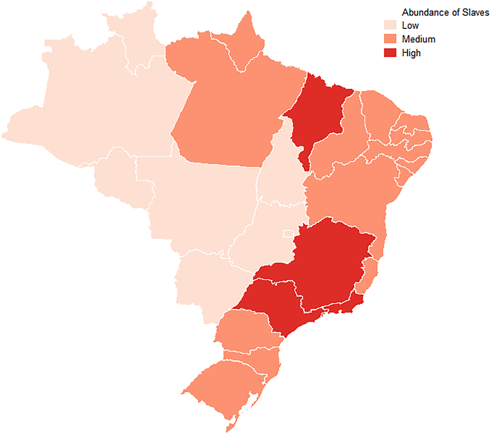
Abundance of slaves, where low, medium and high equals to 1, 2 and 3, respectively. Source: elaboration of the authors; IBGE.

Turnover costs, where low, medium and high equals to 1, 2 and 3, respectively. Source: elaboration of the authors; IBGE.

Cost of sticks, with the distance between the country capital, Município Neutro, and each state capital. Modern borders adapted to the borders in 1872. Source: elaboration of the authors; IBGE.

Prevalence of slavery along the task complexity continuum given β and γ – Men including domestic service.

Prevalence of slavery along the task complexity continuum given β and γ – Women including domestic service.
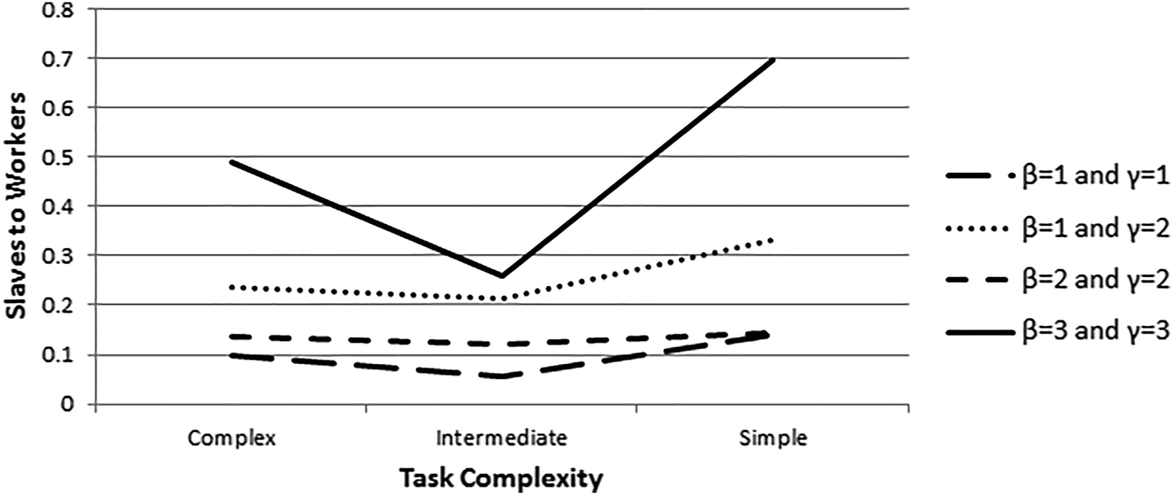
Prevalence of slavery along the task complexity continuum given β and γ – Total including domestic service. (This figure reproduces Figure 1 in the main text.)
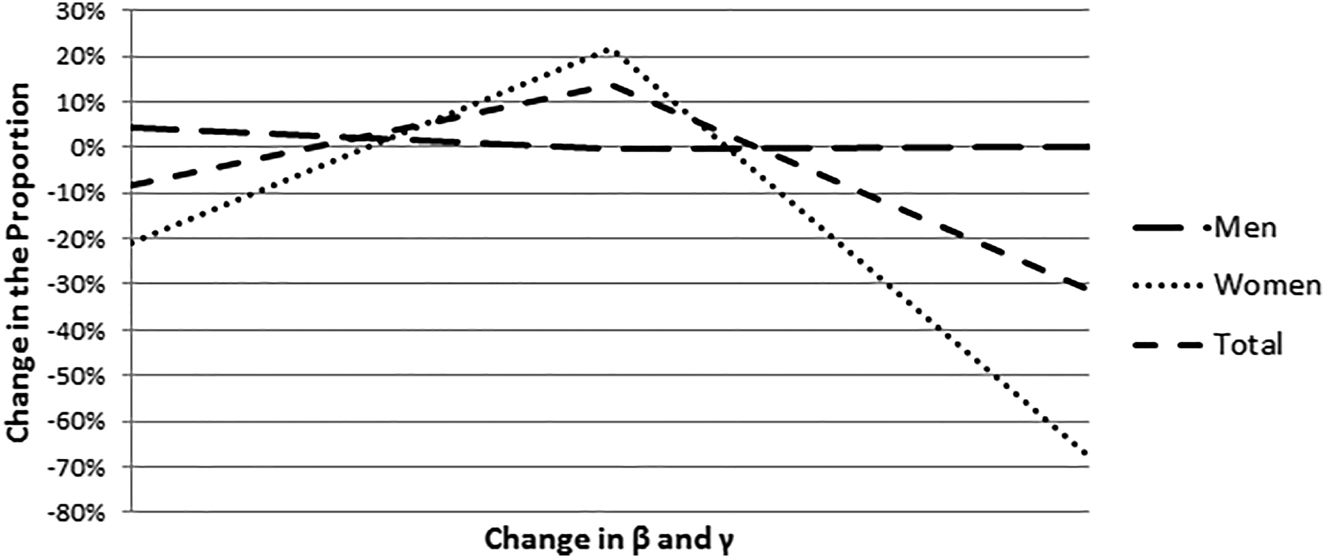
Proportion of slaves in complex tasks to those in simple tasks along β and γ – including domestic service.

Threshold in the change of slaves’ welfare along β and γ – including domestic service.

Threshold in the change of slaves’ welfare along k – including domestic service.
References
Abatino, B., Dari-Mattiacci, G., and Perotti, E. (2011). Depersonalization of business in ancient Rome. Oxf. J. Leg. Stud. 31: 365–389. https://doi.org/10.1093/ojls/gqr001.Search in Google Scholar
Acemolgu, D. and Wolitzky, A. (2011). The economics of labor coercion. Econometrica 79: 555–600.10.3982/ECTA8963Search in Google Scholar
Aubert, J.-J. (1994). Business managers in ancient Rome. E. J. Brill, Leiden.10.1163/9789004450561Search in Google Scholar
Baptist, E.E. (2014). The half has never been told: slavery and the making of American capitalism. New York, Basic Books, a member of the Perseus Books Group.Search in Google Scholar
Barcia, M. and Childs, M.D. (2010). Cuba. In: Paquette, R.L. and Smith, M.M. (Eds.), The Oxford handbook of slavery in the Americas. Oxford University Press, Oxford, pp. 90–110.Search in Google Scholar
Belser, P. (2008). The economics of slavery, forced labor and human trafficking. In: Working paper version for the the encyclopedia of law and economics.10.4337/9781781953068.00026Search in Google Scholar
Blanchard, P. (2010). Spanish South American mainland. In: Paquette, R.L. and Smith, M.M. (Eds.), The Oxford handbook of slavery in the Americas. Oxford University Press, Oxford, pp. 68–89.Search in Google Scholar
Bradley, K. (2011). Slavery in the Roman Republic. In: Bradley, K. and Cartledge, P. (Eds.), The Cambridge world history of slavery, 1: The ancient Mediterranean world. Cambridge University Press, Cambridge, pp. 241–264.10.1017/CHOL9780521840668.014Search in Google Scholar
Burnard, T. (2010). British West Indies and Bermuda. In: Paquette, R.L. and Smith, M.M. (Eds.), The Oxford handbook of slavery in the Americas. Oxford University Press, Oxford, pp. 134–153.Search in Google Scholar
Chwe, M.S.-Y. (1990). Why were workers whipped? Pain in a principal-agent model. Econ. J. 100: 1109–1121. https://doi.org/10.2307/2233961.Search in Google Scholar
Coclanis, P. (2010). Economics of slavery. In: Paquette, R.L. and Smith, M.M. (Eds.), The Oxford handbook of slavery in the Americas. Oxford University Press, Oxford, pp. 489–512.Search in Google Scholar
Coleman, A.N. and Hutchinson, W.K. (2006). Determinants of slave prices: Louisiana, 1725 to 1820. In: Vanderbilt University Department of Economics Working Papers 0624, Vanderbilt University Department of Economics.Search in Google Scholar
Dari-Mattiacci, G. (2013). Slavery and information. J. Econ. Hist. 73: 79–116. https://doi.org/10.1017/s002205071300003x.Search in Google Scholar
Davies, J.K. (2007). Classical Greece: production. In: Scheidel, W., Morris, I., and Saller, R. (Eds.), The Cambridge economic history of the Greco-Roman world. Cambridge University Press, Cambridge, pp. 333–361.10.1017/CHOL9780521780537.013Search in Google Scholar
Davis, Kenneth C. (2016). In the shadow of liberty the hidden history of slavery four presidents and five black lives. Henry Holt and Company, New York.Search in Google Scholar
Dell, M. (2010). The persistent effects of Peru’s mining mita. Econometrica 78: 1863–1903.10.2139/ssrn.1596425Search in Google Scholar
den Heijer, H. (2010). Dutch Caribbean. In: Paquette, R.L. and Smith, M.M. (Eds.), The Oxford handbook of slavery in the Americas. Oxford University Press, Oxford, pp. 154–172.Search in Google Scholar
Domar, E.D. (1970). The causes of slavery or serfdom: a hypothesis. J. Econ. Hist. 30: 18–32. https://doi.org/10.1017/s0022050700078566.Search in Google Scholar
Esposito, E. (2015). Side effects of immunities: the African Slave Trade. Working Paper, EUI MWP, 2015/09.Search in Google Scholar
Fenoaltea, S. (1984). Slavery and supervision in comparative perspective: a model. J. Econ. Hist. 44: 635–668. https://doi.org/10.1017/s0022050700032307.Search in Google Scholar
Fogel, W. (1989). Without consent or contract: the rise and fall of American slavery. Norton, New York, NY.Search in Google Scholar
Fogel, R.W. and Engerman, S.L. (1974). Time on the cross: the economics of American Negro slavery. Wildwood House, London.Search in Google Scholar
Forret, J. (2010). Early Republic and Antebellum United States. In: Paquette, R.L. and Smith, M.M. (Eds.), The Oxford handbook of slavery in the Americas. Oxford University Press, Oxford, pp. 227–248.Search in Google Scholar
Fragoso, J. and Rios, A. (2011). Slavery and politics in colonial Portuguese America: the sixteenth to the eighteenth centuries. In: Eltis, D. and Engerman, S.L. (Eds.), The Cambridge world history of slavery volume 3: AD 1420-AD 1804. Cambridge University Press, Cambridge, pp. 350–377.10.1017/CHOL9780521840682.016Search in Google Scholar
Frier, B.W. and Kehoe, P. (2007). Law and economic institutions. In: Scheidel, W., Morris, I., and Saller, R. (Eds.), The Cambridge economic history of the Greco-Roman world. Cambridge University Press, Cambridge, pp. 113–143.10.1017/CHOL9780521780537.006Search in Google Scholar
Gamauf, R. (2016). Slavery: social position and legal capacity. In: Du Plessis, P.J., Ando, C., and Tuori, K. (Eds.), The Oxford handbook of Roman law and society. Oxford University Press, Oxford, pp. 386–401.10.1093/oxfordhb/9780198728689.013.30Search in Google Scholar
Gardner, J.F. (2011). Slavery and Roman law. In: Bradley, K. and Cartledge, P. (Eds.), The Cambridge world history of slavery, 1: The ancient Mediterranean world. Cambridge University Press, Cambridge, pp. 414–437.10.1017/CHOL9780521840668.021Search in Google Scholar
Garrigus, J. (2010). French Caribbean. In: Paquette, R.L. and Smith, M.M. (Eds.), The Oxford handbook of slavery in the Americas. Oxford University Press, Oxford, pp. 173–200.Search in Google Scholar
Hanes, C. (1996). Turnover cost and the distribution of slave labor in Anglo-America. J. Econ. Hist. 56: 307–329. https://doi.org/10.1017/s0022050700016466.Search in Google Scholar
Harper, K. (2010). Slave prices in late antiquity (and in the very long run). Historia 59: 206–238.10.25162/historia-2010-0013Search in Google Scholar
Harris, W.V. (2007). The late Republic. In: Scheidel, W., Morris, I., and Saller, R. (Eds.), The Cambridge economic history of the Greco-Roman world. Cambridge University Press, Cambridge, pp. 511–540.10.1017/CHOL9780521780537.020Search in Google Scholar
Herbst, J.I. (2000). States and power in Africa: comparative lessons in authority and control. Princeton University Press, Princeton, NJ.Search in Google Scholar
Higman, B.W. (1995). Slave populations of the British Caribbean 1807-1834. The Press University of the West Indies, Kingston, Jamaica.Search in Google Scholar
Joshel, S.R. (1992). Work, identity, and legal studies at Rome: a study of the occupational inscriptions. University of Oklahoma Press, Norman.Search in Google Scholar
Kehoe, D.P. (2007). The early Roman empire: production. In: Scheidel, W., Morris, I., and Saller, R. (Eds.), The Cambridge economic history of the Greco-Roman world. Cambridge University Press, Cambridge, pp. 543–569.10.1017/CHOL9780521780537.021Search in Google Scholar
Klein, H.S. and Vinson, B.III. (2007). African slavery in Latin America and the Caribbean. Oxford University Press, New York, NY.10.1093/oso/9780195189414.001.0001Search in Google Scholar
Lagerlöf, N.P. (2009). Slavery and other property rights. Rev. Econ. Stud. 76: 319–342. https://doi.org/10.1111/j.1467-937x.2008.00511.x.Search in Google Scholar
Lagerlöf, N.P. (2016). Born free. J. Dev. Econ. 121: 1–10. https://doi.org/10.1016/j.jdeveco.2016.02.001.Search in Google Scholar
Littlefield, D.C. (2010). Colonial and revolutionary United States. In: Paquette, R.L. and Smith, M.M. (Eds.), The Oxford handbook of slavery in the Americas. Oxford University Press, Oxford, pp. 201–226.Search in Google Scholar
Lo Cascio, E. (2007). The early empire: the state and the economy. In: Scheidel, W., Morris, I., and Saller, R. (Eds), The Cambridge economic history of the Greco-Roman world. Cambridge University Press, Cambridge, pp. 619–648.10.1017/CHOL9780521780537.024Search in Google Scholar
Lohse, K.R. (2010). Mexico and Central America. In: Paquette, R.L. and Smith, M.M. (Eds.), The Oxford handbook of slavery in the Americas. Oxford University Press, Oxford, pp. 46–67.Search in Google Scholar
Morgan, P.D. (2011). Slavery in the British Caribbean. In: Eltis, D. and Engerman, S.L. (Eds.), The Cambridge world history of slavery volume 3: AD 1420-AD 1804. Cambridge University Press, Cambridge, pp. 378–406.10.1017/CHOL9780521840682.017Search in Google Scholar
Morley, N. (2011). Slavery under the principate. In: Bradley, K. and Cartledge, P. (Eds.), The Cambridge world history of slavery, 1: The ancient Mediterranean world. Cambridge University Press, Cambridge, pp. 265–286.10.1017/CHOL9780521840668.015Search in Google Scholar
Morris, T.D. (1999). Southern slavery and the law, 1619-1860. University of North Carolina Press, Chapel Hill.Search in Google Scholar
Mouritsen, H. (2016). Manumission. In: Du Plessis, P.J., Ando, C., and Tuori, K. (Eds.), The Oxford handbook of Roman law and society. Oxford University Press, Oxford, pp. 402–418.10.1093/oxfordhb/9780198728689.013.31Search in Google Scholar
Naidu, S. and Yuchtman, N. (2013). Coercive contract enforcement: law and the labor market in nineteenth century Industrial Britain. Am. Econ. Rev. 103: 107–144. https://doi.org/10.1257/aer.103.1.107.Search in Google Scholar
Nunn, N. (2008). The long-term effects of Africa’s slave trades. Q. J. Econ. 123: 139–176. https://doi.org/10.1162/qjec.2008.123.1.139.Search in Google Scholar
Paquette, R.L. and Smith, M.M. (2010). The Oxford handbook of slavery in the Americas. Oxford University Press, Oxford.Search in Google Scholar
Peabody, S. (2011). Slavery, freedom, and the law in the Atlantic World, 1420-1807. In: Eltis, D. and Engerman, St.L. (Eds.), The Cambridge world history of slavery volume 3: AD 1420-AD 1804. Cambridge University Press, Cambridge, pp. 594–630.10.1017/CHOL9780521840682.025Search in Google Scholar
Phillips, W.D.Jr (2011). Slavery in the Atlantic Islands and the early modern Spanish Atlantic World. In: Eltis, D. and Engerman, S.L. (Eds.), The Cambridge world history of slavery volume 3: AD 1420-AD 1804. Cambridge University Press, Cambridge, pp. 325–349.10.1017/CHOL9780521840682.015Search in Google Scholar
Rediker, M. (2008). The slave ship: a human history. John Murray, London.Search in Google Scholar
Richardson, D. (2011). Involuntary migration in the early modern world, 1500-1800. In: Eltis, D. and Engerman, S.L. (Eds.), The Cambridge world history of slavery volume 3: AD 1420-AD 1804. Cambridge University Press, Cambridge, pp. 563–593.10.1017/CHOL9780521840682.024Search in Google Scholar
Rihll, T. (2008). Slavery and technology in pre-industrial contexts. In: Lago, E.D. and Katsari, C. (Eds.), Slave systems: ancient and modern. Cambridge University Press, Cambridge, pp. 127–147.10.1017/CBO9780511482748.005Search in Google Scholar
Rodarte, M.M.S. and Júnior, J.M.d. (2008). A estrutura ocupacional revisitada: uma proposta de correção dos dados do Recenseamento Geral do Império de 1872. In: Work presented at XIII seminar about the Mineira economy at Diamantina. Brazil.Search in Google Scholar
Ruef, M. (2012). Constructing labor markets: the valuation of black labor in the U.S. South, 1831 to 1867. Am. Socio. Rev. 77: 970–998. https://doi.org/10.1177/0003122412465282.Search in Google Scholar
Scarano, F.A. (2010). Spanish Hispaniola and Puerto Rico. In: Paquette, R.L. and Smith, M.M. (Eds.), The Oxford handbook of slavery in the Americas. Oxford University Press, Oxford, pp. 21–45.Search in Google Scholar
Scheidel, W. (2008). The comparative economics of slavery in the Greco-Roman world. In: Dal Lago, E. and Katsari, C. (Eds.), Slave systems: ancient and modern. Cambridge University Press, Cambridge, pp. 105–126.10.1017/CBO9780511482748.004Search in Google Scholar
Scheidel, W. (2011). The Roman slave supply. In: Bradley, K. and Cartledge, P. (Eds.), The Cambridge world history of slavery, 1: The ancient Mediterranean world. Cambridge University Press, Cambridge, pp. 287–310.10.1017/CHOL9780521840668.016Search in Google Scholar
Schmidt-Nowara, C. (2010). Emancipation. In: Paquette, R.L. and Smith, M.M. (Eds.), The Oxford handbook of slavery in the Americas. Oxford University Press, Oxford, pp. 578–597.Search in Google Scholar
Scott, R.J., Augusto de Andrade Barbosa, L., and Henrique Borlido Haddad, C. (2017). How does the law put a historical analogy to work?: Defining the imposition of “a condition analogous to that of a slave” in modern Brazil. Duke Journal of Constitutional Law and Public Policy 13: 1–46.10.2139/ssrn.3058191Search in Google Scholar
Scott, R.J. and Venegas, C. (2019). María Coleta and the Capuchin Friar: slavery, salvation, and the adjudication of status (Havana, 1817). William Mary Q 1.10.5309/willmaryquar.76.4.0727Search in Google Scholar
Stauffer, J. (2010). Abolition and antislavery. In: Paquette, R.L. and Smith, M.M. (Eds.), The Oxford handbook of slavery in the Americas. Oxford University Press, Oxford, pp. 556–577.Search in Google Scholar
Temin, P. (2013). The Roman market economy. Princeton: Princeton University Press.10.23943/princeton/9780691147680.001.0001Search in Google Scholar
Tomlin, C. (2010). Freedom bound: law, labor, and civic identity in colonizing English America, 1580-1865. Cambridge University Press, Cambridge.10.1017/CBO9780511778575Search in Google Scholar
Walsh, L.S. (2011). Slavery in the North American mainland colonies. In: Eltis, D. and Engerman, S.L. (Eds.), The Cambridge world history of slavery volume 3: AD 1420-AD 1804. Cambridge University Press, Cambridge, pp. 407–430.10.1017/CHOL9780521840682.018Search in Google Scholar
Watson, J.L. (1980). Asian and African systems of slavery, Blackwell, Oxford.Search in Google Scholar
Watson, A. (2009). The Digest of Justinian. University of Pennsylvania Press, Philadelphia.Search in Google Scholar
Whitman, T.S. (1997). The price of freedom: slavery and manumission in Baltimore and early national Maryland. The University Press of Kentucky, Lexington.Search in Google Scholar
Wiedemann, T. (1981). Greek and Roman slavery. London: Croom Helm.Search in Google Scholar
Wood, K.E. (2010). Gender and slavery. In: Paquette, R.L. and Smith, M.M. (Eds.), The Oxford handbook of slavery in the Americas. Oxford University Press, Oxford, pp. 513–534.Search in Google Scholar
Wright, G. (2006). Slavery and American economic development. Louisiana State University Press, Baton Rouge, LA.Search in Google Scholar
Classical Sources
Roman Law Digests from Watson. (2009). Digest 1.5.3; Digest 1.5.4.1; Digest 1.5.5; Digest 9.2.2 pr; Digest 38.1.26.Search in Google Scholar
Other Sources
Anti-Slavery International, Available at: www.antislavery.org.Search in Google Scholar
Brazilian Census of 1872. Library of the Brazilian Institute of geography and statistics (IBGE), Available at: biblioteca.ibge.gov.br.Search in Google Scholar
The Economist. 2015, March 14th.Search in Google Scholar
The Nation. 2014, September 16th.Search in Google Scholar
The Trans-Atlantic Slave Trade Database, Available at: slavevoyages.org.Search in Google Scholar
United Nations Convention on Slavery, Available at: www.ohchr.org.Search in Google Scholar
Protocol to prevent, suppress and punish trafficking in persons, especially women and children, supplementing the United Nations convention against transnational organized crime, Available at: www.osce.org/odihr/.Search in Google Scholar
© 2021 Giuseppe Dari-Mattiacci and Guilherme de Oliveira published by De Gruyter, Berlin/Boston
This work is licensed under the Creative Commons Attribution 4.0 International License.
Articles in the same Issue
- Frontmatter
- Articles
- Slavery versus Labor
- A Theory of ‘Too Big To Jail’
- A Simple Model of Corporate Fiduciary Duties: With an Application to Corporate Compliance
- Trading with the Dead
- Integration of Complementary Multiproduct Firms
- Optimal Enforcement for Content Industries under Positive External Effects of Piracy