Rapid microwave synthesis of magnetic nanoparticles in physiological serum

Introduction

For several decades, nanoparticles (NPs) have been used in different fields such as energy storage [1], depollution [2], biomedical applications [3], [4], [5], [6]. Indeed, thanks to their size between 1 and 100 nm, comparable to the size of cells, viruses, proteins, interaction between them allows to a great potential for these applications [7]. NPs are indeed used for applications in diagnostic (for example, as a contrast agent CA [8, 9]), in therapy (hyperthermia [10, 11]) or both (for example, with a drug delivery to treat cancer [12, 13]) but the composition of these NPs can be different and adapted according to the targeted application. For example, silver NPs are used as antibacterial agents [14], magnetic NPs such as iron oxide or gadolinium complexes are used as CA [5, 9, 15].

CA allow to enhance image contrast and also to decrease the analysis time in MRI (Magnetic Resonance Imaging). The first CAs were developed during the 60s by Gramiak and Shah [16]. Then, during the 80s, several commercial CAs have been developed with a gadolinium core. Indeed, thanks to the magnetic behaviour of gadolinium Gd³⁺ (paramagnetism), the longitudinal relaxation time T₁ decreases and the image contrast is improved. However, Gd³⁺ is neurotoxic: an organic layer around the inorganic core is mandatory to avoid a neurocellular destruction [17]. Superparamagnetic NPs are used to shorten the transverse relaxation time T₂.

Superparamagnetic Iron Oxide Nanoparticles (SPIONs) such as magnetite (Fe₃O₄) or its oxidized form maghemite (γ-Fe₂O₃) are commonly used as CA [5, 9, 13, 18], [19], [20], [21]. Indeed, SPIONs are biocompatible and different synthesis are well known. To use SPIONs as CA, NPs must be in an aqueous solution, with a narrow size distribution, with a good crystallinity and good magnetic properties. The different synthesis of SPIONs allow to obtain a part of these properties. For example, the coprecipitation is a synthesis directly in an aqueous media with soft conditions but with a possible aggregation of NPs and a large size distribution [22], [23], [24]. To decrease this phenomena, an addition of a ligand during the synthesis can be used: different ligands have been added like for example citric acid [25], [26], [27], polyvinyl alcohol (PVA) [28], oleic acid [29], ethylene glycol [30].

Other synthesis allow to obtain SPIONs directly in water, such as hydrothermal synthesis [31] or microemulsion [32] but the conditions are hard and don’t allow to obtain monodisperse NPs. The thermal decomposition is an alternative to synthesize SPIONs and presents the advantage of obtaining SPIONs which are monodisperse, with a narrow size distribution and a good crystallinity [33, 34]. By thermal decomposition at high temperature, synthesized SPIONs are stable in an organic solution (cyclohexane, chloroform, toluene, …), but a subsequent phase transfer step is therefore mandatory to use SPIONs for the biomedical applications [35, 36].

To obtain monodisperse SPIONs in an aqueous media, a new synthesis is more and more used: the microwave synthesis [27, 37], [38], [39]. Indeed, thanks to the microwave irradiations, the temperature is better controlled inside the reactor: there is a vibration of the solvent molecules generating local heating of the solution. Synthesized SPIONs are stable in an aqueous solution, monodisperse (because a ligand was added during the synthesis), with a good crystallinity and good magnetic properties.

Numerous studies describe the potential use of SPIONs but generally synthesized in ultra-pure water or dispersed in water after a phase transfer. However, in a living organism, there are several proteins and molecules which can lead to an aggregation of these NPs. To limit this phenomenon, we consider it important to obtain SPIONs that are stable in a physiological medium before application.

The goal of this study is to compare the synthesis of SPIONs in different aqueous media. Indeed, we compare a synthesis in ultra-pure water to a synthesis in physiological serum and to a redispersion of SPIONs in a physiological serum. For each synthesis, systematic characterizations are realized to determine the size, the crystallinity, the composition and the magnetic properties. Then, a comparison of relaxivity values of these different synthesis is performed to verify the influence of the physiological serum on the synthesis.

Experimental

Results and discussions

Figure 1 shows the micrographs of NPs_ww (Fig. 1a), NPs_wp (Fig. 1c) and NPs_pp (Fig. 1e). For the three samples, the shape of SPIONs is spherical. To obtain the mean diameter, a fit by a gaussian function is carried out. The mean diameter is equal to 2.67 ± 0.76, 3.00 ± 0.94 and 3.19 ± 1.20 nm for NPs_ww, NPs_wp and NPs_pp respectively thanks to the size distribution of each samples, obtained with a lower magnification (Fig. 1b, d and f). The size distribution obtained with the NPs synthesised and dispersed in water is narrower than for the synthesis or redispersion in physiological serum: the presence of NaCl in physiological serum increases the mean diameter. In addition, with the physiological serum, a little aggregation of NPs appears due to the presence of NaCl. Indeed, a NaCl matrix encompasses SPIONs. This matrix is weak when SPIONs are just dispersed in physiological serum after synthesis in water (Fig. 1c) and it is more important when the synthesis and the dispersion are in this serum (Fig. 1e): the size distribution is so more important in NaCl solution that in ultra-pure water.

Fig. 1:

TEM images of NPs_ww (a), NPs_wp (c) and NPs_pp (e) with their size distribution histograms respectively in (b), (d) and (f). The black curve on each histogram represents a fit by a gaussian function.

To confirm this hypothesis, a DLS measurement is carried out. For that, the solution of each NPs was analysed to determine the hydrodynamic diameter as well as the stability of NPs (Fig. 2). Indeed, the hydrodynamic diameter is the diameter of the inorganic core increased by the thickness of the organic layer and the solvation sphere. The DLS measurements are expressed in number to be compared with the obtained TEM results. The mean hydrodynamic diameter of samples (determined by a log-normal fit) is equal to 7 ± 2 nm for NPs_ww, 11 ± 3 nm for NPs_wp and 10 ± 2 nm for NPs_pp: these values are higher that the diameter obtained by TEM measurements confirming the presence of an organic layer. In addition, as shown in the TEM micrographs of NPs_wp and NPs_pp (Fig. 1c and e), an aggregation of SPIONs is present and increases the value of the hydrodynamic diameter: it is the reason that the hydrodynamic diameter of NPs_wp and NPs_pp are higher than the hydrodynamic diameter of NPs_ww. Finally, the presence of the NaCl matrix can increase to a little the mean hydrodynamic diameter in agreement with TEM observations. To confirm the presence of this NaCl matrix, XRD measurements are carried out.

Fig. 2:

DLS measurements of NPs_ww (blue), NPs_wp (green) and NPs_pp (pink) as function of number of NPs.

Then, a XRD measurement is performed to describe the inorganic core and precisely the crystallographic structure (Fig. 3). Indeed, it exists two types of SPIONs which are magnetite Fe₃O₄ and maghemite γ-Fe₂O₃. These two iron oxide compositions crystallize in the same inverse spinel structure (Fd3‾m). The lattice parameter is equal to 8.385 and 8.354 Å for magnetite and maghemite respectively. XRD patterns of each samples are compared with a reference pattern of magnetite (COD: 9005836). For the three samples, the main diffraction peaks of magnetite, i.e. (200), (311), (400), (511) and (440), are present.

Fig. 3:

XRD patterns of NPs_ww (blue), NPs_wp (green) and NPs_pp (pink) with a comparison of reference patterns of magnetite Fe₃O₄ (COD 9005836) and sodium chloride NaCl (COD 231042).

The lattice parameter is calculated for each sample thanks to these main peaks and it is equal to 8.38, 8.36 and 8.37 Å for NPs_ww, NPs_wp and NPs_pp respectively. These calculated lattice parameters are between those of magnetite and maghemite: the synthesized NPs for this study correspond to Fe_3−δO₄ sub-stoichiometric magnetite with δ the stoichiometric deviation. Using XRD patterns, the crystallite size can be calculated thanks to the Debye-Scherrer equation which is t = (kλ)/(βcosθ) where t is the size of the crystallite, λ the wavelength of the X-ray radiation, β the FWHM of the main peak with a correction and θ the Bragg angle. The crystallite size is similar to the diameter obtained with the TEM for the three sample: 3.3, 3.7 and 3.6 nm respectively for NPs_ww, NPs_wp and NPs_pp.

In addition, for NPs_wp and NPs_pp, several peaks are present and correspond to a NaCl phase (COD: 231042) in agreement with the interpretation of the matrix and slight aggregation observed on TEM micrographs (Fig. 1c and e) as resulting from the use of physiological serum containing NaCl. To confirm the presence or the absence of NaCl in each sample as function of aqueous solvent and to determine the oxidation state of iron in the inorganic core, Raman spectroscopy measurements are carried out.

The Raman spectra are illustrated on Fig. 4. For the three samples, we observe the vibrational modes of Fe₃O₄: E_g at 300 cm⁻¹, T_2g at 540 cm⁻¹ and A_1g at 670 cm⁻¹ [42]. This last mode is characteristic of the oxidation state of the iron oxide: a narrow band is representative of magnetite and a large band from 660 to 720 cm⁻¹ with a split of this mode into two components is representative of maghemite. For the three samples, we can see an enlargement with the appearance of a shoulder for the A_1g mode by comparison with the magnetite spectrum. This observation implying an oxidation of the nanoparticles without a complete split characteristic of the unique presence of maghemite confirm the synthesis of Fe_3−δO₄ sub-stoichiometric magnetite for all samples as determined by XRD measurements. In addition, for NPs_wp and NPs_pp, the presence of NaCl is confirmed with the Raman spectroscopy. Indeed, several bands are present at 425, 1257, 1323, 1385 and 1660 cm⁻¹ and are similar with the bands on a NaCl spectrum (Fig. 4).

Fig. 4:

Raman spectra of NPs_ww (blue), NPs_wp (green) and NPs_pp (pink) obtained with a laser at 633 nm at room temperature compared to a magnetite reference Fe₃O₄ and a sodium chloride reference NaCl.

Then, the magnetic properties of each sample are analysed to determine the magnetic state and the saturation magnetization (Fig. 5). For this goal, the evolution of the magnetic moment M (emu g⁻¹) in function of magnetic field H (Oe) is analysed at 300 K and at 5 K. Indeed, at room temperature (Fig. 5a), the superparamagnetic state can be determined thanks to the presence of a hysteresis or not: without hysteresis, NPs are in a superparamagnetic state; with hysteresis, NPs are in a permanent magnetic state such as ferrimagnetic, ferromagnetic or antiferromagnetic. For the three samples studied here, the absence of hysteresis indicates the superparamagnetic state. With this curve, the magnetization saturation can be determined: it is equal to 55, 29 and 31 emu g⁻¹ for NPs_ww, NPs_wp and NPs_pp respectively. The presence of NaCl in NPs_wp and in NPs_pp decreases the magnetization saturation because NaCl is a diamagnetic compound: iron oxide nanoparticles are surrounded by a NaCl matrix.

Fig. 5:

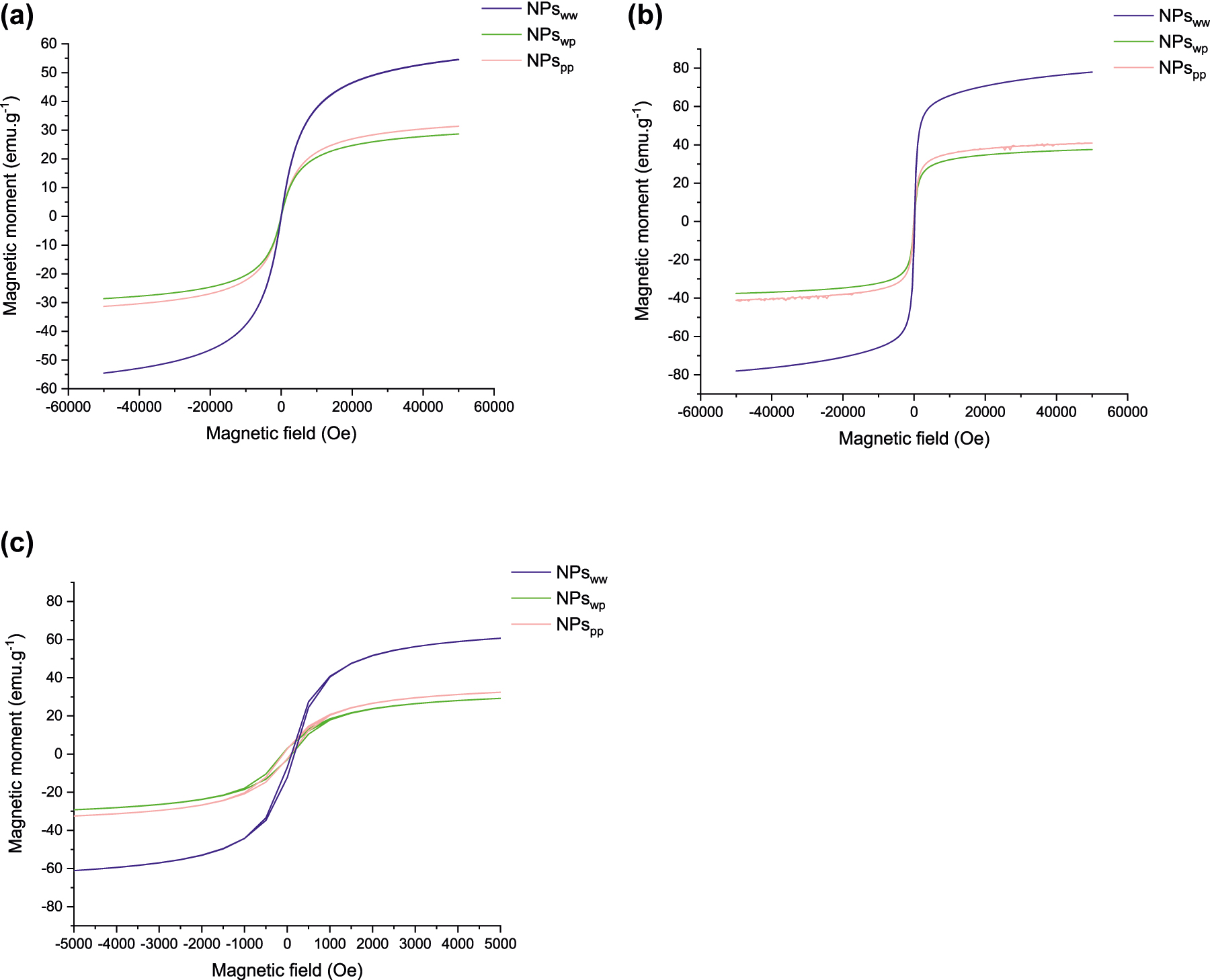
Magnetic moment (emu g⁻¹) as function of magnetic field (Oe) for NPs_ww (blue), NPs_wp (green) and NPs_pp (pink) at 300 K (a), at 5 K (b) and a zoom at 5 K (c).

To confirm the superparamagnetic state, a magnetic measurement at 5 K is carried out (Fig. 5b). At this temperature, the magnetic moment on iron oxide is in a blocked state so the magnetic behaviour is similar to a cooperative magnetism thus generating a hysteresis in the magnetic curves (Fig. 5c). The magnetization saturation obtained at 5 K is higher to the magnetization saturation at 300 K du to the blocked state of the magnetic moment: it is equal to 78, 38 and 41 emu g⁻¹ for NPs_ww, Nps_wp and NPs_pp respectively.

To complete magnetic characterizations, a ZFC-FC (Zero Field Cooled – Field Cooled) measurement is carried out to determine the blocking temperature T_B: this temperature is the transition between the superparamagnetic state and the blocked state (Fig. 6). Several methods exist to determine exactly the value of T_B with a ZFC-FC curve [43]. The most used is an assimilation to the maximum of the ZFC curve (it is the curve from 5 to 300 K). For each sample, the determined T_B is 14, 25 and 21 K for NPs_ww, Nps_wp and NPs_pp respectively: all samples present a superparamagnetic state at room temperature. In addition, the ZFC-FC curves can be considered as a T_B distribution. For an aggregation of NPs or a larger size distribution, the curve will be larger while for a narrow size distribution of NPs, the curve will be narrower. In agreement, the ZFC curve is narrow for NPs_ww and larger for NPs_wp and NPs_pp. For these two samples, the distribution increase is due to the presence of the NaCl matrix. Indeed, this matrix encapsulates iron oxide nanoparticles thus creating a set of nanoparticles: this set has a higher size compared to a single nanoparticle according to a magnetic point of view with a collective behaviour.

Fig. 6:

Magnetic moment as function the temperature measured under a magnetic field (200 Oe) of NPs_ww (blue), NPs_wp (green) and NPs_pp (pink).

Finally, for the application of SPIONs as contrast agents in MRI, the value of relaxivity r_i (s⁻¹ mmol⁻¹ L) has to be evaluated. This is done by measuring the relaxation rate R_i (i = 1;2) as a function of SPIONs concentration (at 37 °C and 1.41 T, Fig. 7). Indeed, the paramagnetic contribution to relaxation is linearly proportional to the concentration of CA according to the equation R_i = r_i*C + (1/T₀) where C is the concentration of SPIONs (mM) and T₀ is the relaxation time of the aqueous solution without paramagnetic agent. The parameter r_i is called proton relaxivity and is given in s⁻¹ mM⁻¹. Here both types of relaxivities, i.e. longitudinal r₁ and transverse r₂, are obtained from the linear fitting of data in Fig. 7 in order to evaluate the efficiency of SPIONS to act as a contrast agent. Concerning longitudinal relaxation, the relaxivity r₁ is 17, 12 and 18 s⁻¹ mmol⁻¹ L for NPs_ww, NPs_wp and NPs_pp respectively. The relaxivity of NPs_wp is slightly lower than equivalent relaxivities of NPs_ww and NPs_pp. However, for the transverse relaxivity r₂, which is known to be the relevant parameter for superparamagnetic iron oxide nanoparticles used as negative contrast agent [8, 9], NPs_wp has a higher value than the others. Indeed, the values are 69, 44 and 51 s⁻¹ mmol⁻¹ L for NPs_wp, NPs_ww and NPs_pp respectively. Compared to a commercial contrast agent (Endorem^®), these values of transverse relaxivity are lower (for Endorem^®, r₁ is between 10 and 24 s⁻¹ mmol⁻¹ L and r₂ is between 100 and 158 s⁻¹ mmol⁻¹ L [44], [45], [46]) but the ratio between r₂ and r₁ is similar. This ratio is a good indicator to determine if a contrast agent is a good candidate for MRI: if this ratio is higher to 2, NPs will be good candidate for MRI [47]. For the Endorem^®, the ratio is between 4 and 15 according to the different authors. This ratio is equal to 2.6, 5.8 and 2.8 for NPs_ww, NPs_wp and NPs_pp respectively: all samples can be good candidates for MRI, particularly NPs_wp with a ratio of 5.8 similar to Endorem^®.

Fig. 7:

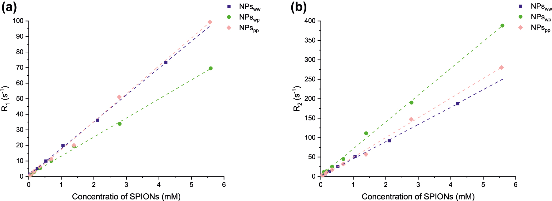
Longitudinal R₁ (a) and transverse R₂ (b) relaxation rate (in s⁻¹) as a function of SPIONs concentration (mM) at 60 MHz and 37 °C for NPs_ww (blue), NPs_wp (green) and NPs_pp (pink). Dashed lines represent the linear regression done for evaluating the relaxivity r_i=1;2.

Conclusion

In summary, thanks to the microwave synthesis, superparamagnetic iron oxide nanoparticles can be synthesised with a small diameter, a good monodispersity and stability in an aqueous solution. These nanoparticles can be used for the biomedical applications with a dispersion in ultra-pure water and in physiological conditions. In this work, for the first time, this synthesis method of SPIONs is performed in ultra-pure water with a validate redispersion in physiological serum (containing 0.9 g of NaCl per 100 mL of ultra-pure water) and a direct synthesis in physiological serum is also realised. The nanoparticles obtained by these different conditions offer a small diameter and a colloidal stability thanks to the microwave use and the introduction of an organic layer (a citrate layer) as surfactant during an one-step synthesis. In addition, the inorganic core is a sub-stoichiometric iron oxide (Fe_3−δO₄) with a good crystallinity and a superparamagnetic state at room temperature. Finally, relaxivity measurements are carried out to conclude that these SPIONs are good candidates for MRI. In particular for the SPIONs synthesised in ultra-pure water and redispersed in physiological serum, the ratio of relaxivity (r₂/r₁) is similar to a ratio from a commercial contrast agent (Endorem^®).

References

[1] J. Peng, W. Zhang, L. Chen, T. Wu, M. Zheng, H. Dong, H. Hu, Y. Xiao, Y. Liu, Y. Liang. Chem. Eng. J.404, 126461 (2021), https://doi.org/10.1016/j.cej.2020.126461.Search in Google Scholar
[2] R. Ortega-Villar, L. Lizárraga-Mendiola, C. Coronel-Olivares, L. D. López-León, C. A. Bigurra-Alzati, G. A. Vázquez-Rodríguez. J. Environ. Manag.242, 487 (2019).10.1016/j.jenvman.2019.04.104Search in Google Scholar PubMed
[3] K. Niemirowicz, K. Markiewicz, A. Wilczewska, H. Car. Adv. Med. Sci.57, 196 (2012), https://doi.org/10.2478/v10039-012-0031-9.Search in Google Scholar PubMed
[4] S. Mornet, S. Vasseur, F. Grasset, E. Duguet. J. Mater. Chem.14, 2161 (2004), https://doi.org/10.1039/b402025a.Search in Google Scholar
[5] L. L. Israel, A. Galstyan, E. Holler, J. Y. Ljubimova. J. Contr. Release320, 45 (2020), https://doi.org/10.1016/j.jconrel.2020.01.009.Search in Google Scholar PubMed PubMed Central
[6] G. Wang, X. Zhang, A. Skallberg, Y. Liu, Z. Hu, X. Mei, K. Uvdal. Nanoscale6, 2953 (2014), https://doi.org/10.1039/c3nr05550g.Search in Google Scholar PubMed
[7] R. Kumar, M. Nayak, G. C. Sahoo, K. Pandey, M. C. Sarkar, Y. Ansari, V. N. R. Das, R. K. Topno, Bhawna, M. Madhukar, P. Das. J. Infect. Chemother.25, 325 (2019), https://doi.org/10.1016/j.jiac.2018.12.006.Search in Google Scholar PubMed
[8] M.-A. Fortin, C. S. S. R. Kumar (Eds.). in Magnetic Characterization Techniques for Nanomaterials, pp. 511–555, Springer Berlin Heidelberg, Berlin, Heidelberg (2017).10.1007/978-3-662-52780-1_15Search in Google Scholar
[9] J. Ward. Radiography13, e54 (2007), https://doi.org/10.1016/j.radi.2006.09.002.Search in Google Scholar
[10] F. Reyes-Ortega, Á. Delgado, G. Iglesias. Nanomaterials11, 627 (2021), https://doi.org/10.3390/nano11030627.Search in Google Scholar PubMed PubMed Central
[11] Z. E. Gahrouei, M. Imani, M. Soltani, A. Shafyei. Adv. Nat. Sci. Nanosci. Nanotechnol.11, 025001 (2020), https://doi.org/10.1088/2043-6254/ab878f.Search in Google Scholar
[12] F. Soetaert, P. Korangath, D. Serantes, S. Fiering, R. Ivkov. Adv. Drug Deliv. Rev.163–164, 65 (2020), https://doi.org/10.1016/j.addr.2020.06.025.Search in Google Scholar PubMed PubMed Central
[13] S. Tong, H. Zhu, G. Bao. Mater. Today31, 86 (2019), https://doi.org/10.1016/j.mattod.2019.06.003.Search in Google Scholar PubMed PubMed Central
[14] J. Gouyau, R. E. Duval, A. Boudier, E. Lamouroux. IJMS22, 1905 (2021), https://doi.org/10.3390/ijms22041905.Search in Google Scholar PubMed PubMed Central
[15] W. Xiaoming, G. Shiwei, L. Zhiqian, X. Xueyang, G. Lei, L. Qiang, Z. Hu, G. Qiyong, L. Kui. Appl. Mater. Today17, 92 (2019), https://doi.org/10.1016/j.apmt.2019.07.019.Search in Google Scholar
[16] R. Gramiak, P. M. Shah. Invest. Radiol., 356 (1968), https://doi.org/10.1097/00004424-196809000-00011.Search in Google Scholar PubMed
[17] T. J. Clough, L. Jiang, K.-L. Wong, N. J. Long. Nat. Commun.10, 1420 (2019), https://doi.org/10.1038/s41467-019-09342-3.Search in Google Scholar PubMed PubMed Central
[18] V. F. Cardoso, A. Francesko, C. Ribeiro, M. Bañobre-López, P. Martins, S. Lanceros-Mendez. Adv. Healthcare Mater.7, 1700845 (2018), https://doi.org/10.1002/adhm.201700845.Search in Google Scholar PubMed
[19] A. Espinosa, R. Di Corato, J. Kolosnjaj-Tabi, P. Flaud, T. Pellegrino, C. Wilhelm. ACS Nano10, 2436 (2016), https://doi.org/10.1021/acsnano.5b07249.Search in Google Scholar PubMed
[20] X. Batlle, C. Moya, M. Escoda-Torroella, Ò. Iglesias, A. F. Rodríguez, A. Labarta. J. Magn. Magn Mater.543, 168594 (2022).10.1016/j.jmmm.2021.168594Search in Google Scholar
[21] E. Taboada, E. Rodríguez, A. Roig, J. Oró, A. Roch, R. N. Muller. Langmuir23, 4583 (2007), https://doi.org/10.1021/la063415s.Search in Google Scholar PubMed
[22] P. Arévalo, J. Isasi, A. C. Caballero, J. F. Marco, F. Martín-Hernández. Ceram. Int.43, 10333 (2017), https://doi.org/10.1016/j.ceramint.2017.05.064.Search in Google Scholar
[23] S. Slimani, C. Meneghini, M. Abdolrahimi, A. Talone, J. P. M. Murillo, G. Barucca, N. Yaacoub, P. Imperatori, E. Illés, M. Smari, E. Dhahri, D. Peddis. Appl. Sci.11, 5433 (2021), https://doi.org/10.3390/app11125433.Search in Google Scholar
[24] K. Petcharoen, A. Sirivat. Mater. Sci. Eng. B177, 421 (2012), https://doi.org/10.1016/j.mseb.2012.01.003.Search in Google Scholar
[25] O. A. Abu-Noqta, A. A. Aziz, A. I. Usman. Mater. Today Proc.17, 1072 (2019).10.1016/j.matpr.2019.06.516Search in Google Scholar
[26] S. Nigam, K. C. Barick, D. Bahadur. J. Magn. Magn Mater.323, 237 (2011), https://doi.org/10.1016/j.jmmm.2010.09.009.Search in Google Scholar
[27] T. Girardet, A. Cherraj, A. Pinzano, C. Henrionnet, F. Cleymand, S. Fleutot. Pure Appl. Chem.93, 1265 (2021), https://doi.org/10.1515/pac-2021-0303.Search in Google Scholar
[28] C. Tao, Y. Chen, D. Wang, Y. Cai, Q. Zheng, L. An, J. Lin, Q. Tian, S. Yang. Nanomaterials9, 699 (2019), https://doi.org/10.3390/nano9050699.Search in Google Scholar PubMed PubMed Central
[29] I. O. Wulandari, H. Sulistyarti, A. Safitri, D. J. D. H. Santjojo, A. Sabarudin. J. Appl. Pharmaceut. Sci.9, 1 (2019).Search in Google Scholar
[30] M. Anbarasu, M. Anandan, E. Chinnasamy, V. Gopinath, K. Balamurugan. Spectrochim. Acta Part A Mol. Biomol. Spectrosc.135, 536 (2015), https://doi.org/10.1016/j.saa.2014.07.059.Search in Google Scholar PubMed
[31] H. Kahil, A. Faramawy, H. El-Sayed, A. Abdel-Sattar. Crystals11, 1153 (2021), https://doi.org/10.3390/cryst11101153.Search in Google Scholar
[32] T. Lu, J. Wang, J. Yin, A. Wang, X. Wang, T. Zhang. Colloids Surf. A Physicochem. Eng. Asp.436, 675 (2013), https://doi.org/10.1016/j.colsurfa.2013.08.004.Search in Google Scholar
[33] A. G. Roca, L. Gutiérrez, H. Gavilán, M. E. Fortes Brollo, S. Veintemillas-Verdaguer, M. D. P. Morales. Adv. Drug Deliv. Rev.138, 68 (2019), https://doi.org/10.1016/j.addr.2018.12.008.Search in Google Scholar PubMed
[34] X. Guo, W. Wang, Y. Yang, Q. Tian. CrystEngComm18, 9033 (2016), https://doi.org/10.1039/c6ce01963c.Search in Google Scholar
[35] O. Bixner, A. Lassenberger, D. Baurecht, E. Reimhult. Langmuir31, 9198 (2015), https://doi.org/10.1021/acs.langmuir.5b01833.Search in Google Scholar PubMed PubMed Central
[36] F. Crippa, L. Rodriguez-Lorenzo, X. Hua, B. Goris, S. Bals, J. S. Garitaonandia, S. Balog, D. Burnand, A. M. Hirt, L. Haeni, M. Lattuada, B. Rothen-Rutishauser, A. Petri-Fink. ACS Appl. Nano Mater.2, 4462 (2019), https://doi.org/10.1021/acsanm.9b00823.Search in Google Scholar
[37] E. Aivazoglou, E. Metaxa, E. Hristoforou. AIP Adv.8, 048201 (2018), https://doi.org/10.1063/1.4994057.Search in Google Scholar
[38] I. Fernández-Barahona, M. Muñoz-Hernando, F. Herranz. Molecules24, 1224 (2019), https://doi.org/10.3390/molecules24071224.Search in Google Scholar PubMed PubMed Central
[39] Y.-J. Liang, Y. Zhang, Z. Guo, J. Xie, T. Bai, J. Zou, N. Gu. Chem. Eur J.22, 11807 (2016), https://doi.org/10.1002/chem.201601434.Search in Google Scholar PubMed
[40] P. Venturini, S. Fleutot, F. Cleymand, T. Hauet, J. Dupin, J. Ghanbaja, H. Martinez, J. Robin, V. Lapinte. ChemistrySelect3, 11898 (2018), https://doi.org/10.1002/slct.201802234.Search in Google Scholar
[41] M. D. Abràmoff, P. J. Magalhães, S. J. Ram. Biophot. Int.36–42 (2004).Search in Google Scholar
[42] M. Hanesch. Geophys. J. Int.177, 941 (2009), https://doi.org/10.1111/j.1365-246x.2009.04122.x.Search in Google Scholar
[43] I. J. Bruvera, P. Mendoza Zélis, M. Pilar Calatayud, G. F. Goya, F. H. Sánchez. J. Appl. Phys.118, 184304 (2015), https://doi.org/10.1063/1.4935484.Search in Google Scholar
[44] N. Ohannesian, C. T. De Leo, K. S. Martirosyan. Mater. Today Proc.13, 397 (2019), https://doi.org/10.1016/j.matpr.2019.03.172.Search in Google Scholar
[45] M. Geppert, M. Himly. Front. Immunol.12, 688927 (2021).10.3389/fimmu.2021.688927Search in Google Scholar PubMed PubMed Central
[46] A. M. Predescu, E. Matei, A. C. Berbecaru, C. Pantilimon, C. Drăgan, R. Vidu, C. Predescu, V. Kuncser. R. Soc. Open Sci.5, 171525 (2018), https://doi.org/10.1098/rsos.171525.Search in Google Scholar PubMed PubMed Central
[47] Y. Gossuin, P. Gillis, A. Hocq, Q. L. Vuong, A. Roch. WIREs Nanomed. Nanobiotechnol.1, 299 (2009), https://doi.org/10.1002/wnan.36.Search in Google Scholar PubMed
© 2022 IUPAC & De Gruyter. This work is licensed under a Creative Commons Attribution-NonCommercial-NoDerivatives 4.0 International License. For more information, please visit: http://creativecommons.org/licenses/by-nc-nd/4.0/
Articles in the same Issue
- Frontmatter
- Special Topic Paper