Room temperature polaritonic soft-spin XY Hamiltonian in organic–inorganic halide perovskites

2.1 Characterization of polaritons in MAPbBr₃

The cavity structure is shown schematically in Figure 1(a). The planar Fabry–Pérot cavity was made by a wafer-bond process of two DBR mirrors. Then, the single-crystal MAPbBr₃ was grown by a solution method under the confinement of the microcavity (∼330 nm). With this method, high-quality, large-sized perovskite single crystals can be grown in the cavity, as shown in Figure 1(b). More details of the fabrications, growth, and characterizations can be found in Methods and our previous work [14]. Figure 1(c) shows the absorption and the PL spectra of the MAPbBr₃ plate grown in the 200-nm thick empty bonded quartz substrates. Previous studies show that excitons in MAPbBr₃ perovskite have an exciton binding energy of about 25–42 meV at room temperature [17], [18], [19], supporting room-temperature excitons. This is consistent with our fitted exciton binding energy of ∼38 meV from the absorption spectrum based on the Elliott model [20], [21] in Figure 1(c).

Figure 1:

Characterization of exciton–polaritons in organic–inorganic halide perovskite microcavity. (a) Schematic of the perovskite microcavity, consisting of a solution-grown MAPbBr₃ single crystal sandwiched between two 12.5 pairs DBR mirrors with cavity quality factor Q ∼700–800. (b) Optical image of a MAPbBr₃ single crystal in the cavity with a transmission illumination. Scale bar: 50 μm. (c) The normalized absorption and photoluminescence (PL) spectra of a ∼200-nm thick MAPbBr₃ single-crystal at room temperature. The absorption spectrum in the top panel was fitted by the Elliott model [20], [21]. An excitonic peak (blue solid line) and a continuum absorption curve (cyan solid line) can be observed clearly. An exciton binding energy of ∼38 meV was extracted. (d) Angle-resolved PL dispersion of the strong-coupled exciton–polariton of the perovskite cavity. The dashed lines are fitted curves of the exciton energy (exciton), cavity mode (cavity), and lower polariton mode (LP).

For the perovskite sample in the cavity, a sharp polariton dispersion can be observed via the angle-resolved PL spectrum shown in Figure 1(d). The polaritons were formed from the strong coupling between the exciton in perovskite and the cavity photons, which can be described very well with a coupled oscillator model neglecting linewidth:

Here, the cavity mode is represented as E cav k ‖ = E 0 + ℏ 2 k ‖ 2 2 m with mode energy E ₀ at k _‖ = 0 and effective mass m of the cavity photon. E _ex is the exciton energy that can be extracted from the absorption spectrum in Figure 1(c). E is the eigenvalue of the polaritons, and a and b represent the Hopfield coefficients. From the fitting results as the dashed lines in Figure 1(d), we extracted the Rabi splitting Ω = 130 meV and a negative exciton–photon detuning of Δ = −96 meV for this sample.

2.2 Room-temperature polariton condensation

The strong nonlinear properties of MAPbBr₃ enable us to achieve polariton condensation. A 450-nm, 250-fs pulsed laser was used to excite the sample nonresonantly with a laser spot size of ∼28 μm. Figure 2(a) shows the angle-resolved power-dependent PL dispersions with pulse energy at 0.1 P _th, P _th, and 1.5 P _th from left to right, where P _th is the threshold of ∼42.2 μJ cm⁻². A pinhole at the real-space imaging plane was used to only extract the PL from the condensation area. Above the threshold, the polariton ground state at k _|| = 0 exhibits a strong nonlinear emission enhancement and linewidth narrowing, clearly evidences of the condensation. This is also illustrated in Figure 2(b) through the PL intensity and linewidth as a function of the pulse energy. Meanwhile, due to the polariton–polariton interactions, polariton dispersion has a continuous blueshift with the increase of density. A stronger blueshift was observed below the threshold due to the strong exciton reservoir interactions. All these typical features demonstrated the occurrence of polariton condensation in our perovskite system.

Figure 2:

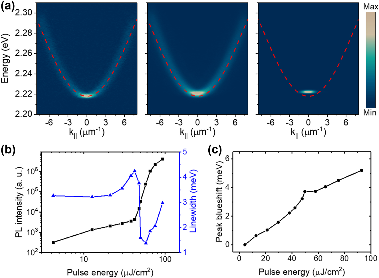
Exciton–polariton condensation at room temperature. (a) Angle-resolved power-dependent PL dispersions under nonresonant excitation at 0.1 P _th, P _th, and 1.5 P _th from left to right, where P _th (∼42.2 μJ cm⁻²) is the pumping power of condensation threshold. With the power increasing, the polaritons condensate at the ground state of the polariton mode. The dashed red lines are the fitted curve of the lower polariton mode with low pumping power. (b) Log–log plot of the integrated PL intensities of the ground polariton mode at k _|| = 0 and the full width at half maximum versus pulse energy. The nonlinear increase of the intensity and the narrowing of the linewidth clearly demonstrate the polariton condensation. (c) PL peak blueshifts of the mode at k _|| = 0. Due to the strong exciton reservoir interactions, a stronger blueshift was observed below the threshold.

2.3 Soft-spin XY Hamiltonian by polariton condensate lattices

By utilizing the long-range coherence of the condensates, we can create multiple condensates and study their interactions. Due to the repulsion interaction between polaritons, condensation can occur at a high energy state with a nonzero in-plane momentum when the pumping laser spot is small [22], [23]. Interference and phase difference synchronization occur when different out-flowing condensates meet according to previous theoretical models and the experimental results [6], [23], [24]. A polariton dyad was used to demonstrate this phase synchronization in our experiment. A phase-only reflective spatial light modulator was used to generate the designed condensate array, and more details of the experimental setup can be found in Methods. As shown in Figure 3, with the separation distances between the two condensates increasing, the interference fringes increase from zero to three, demonstrating the transitions from antiphase to the in-phase and back to the antiphase synchronization between the two condensates. The red arrows marked at the condensates represent the relative phase directions. The corresponding PL dispersions in Figure 3(b) also demonstrate these different phase synchronizations.

Figure 3:

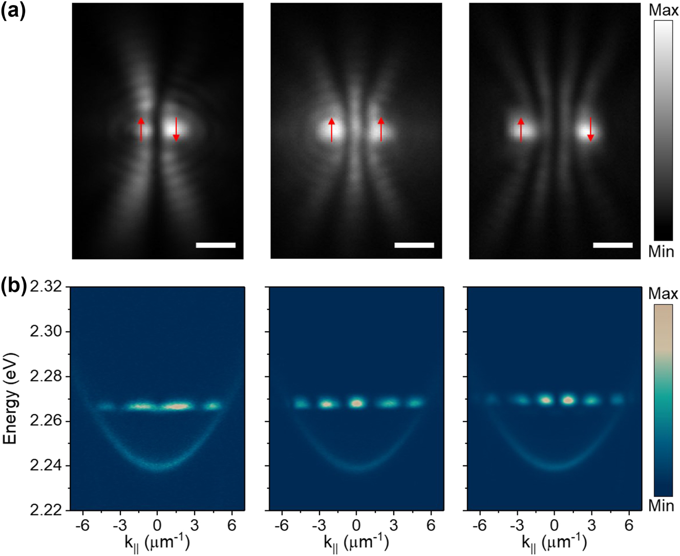
Phase configuration between two polariton condensates. (a) The time-integrated real-space images of the two polariton condensates with different separation distances of 1.78, 2.5, and 3.55 μm from left to right, respectively. With the separation distances increase, the interference fringes increase from zero to three, demonstrating the transitions from antiphase to the in-phase and back to the antiphase synchronization between the two condensates. The red arrows marked at the condensates represent the relative spin directions. Scale bars: 2 μm. (b) The corresponding angle-resolved PL dispersions of the condensates in (a). The detuning of this sample is smaller than that shown in Figure 2. The interference fringes at high energy state also demonstrate the different phase synchronizations between the two condensates.

To validate the capability of our sample to construct a large-scale polariton condensate lattice, we assembled a 2 × 2 square lattice to simulate the two-dimensional soft-spin XY Hamiltonian. As shown in Figure 4(a), one interference fringe can be observed between the nearest condensates, demonstrating the in-phase coupling and the ferromagnetic states. Like the one-dimensional cases in Figure 3, with the separation distance increase between the condensates, antiferromagnetic and the next ferromagnetic coupling states can be obtained from the even and odd interference fringes between the nearest condensates in Figure 4(b) and (c), respectively.

Figure 4:

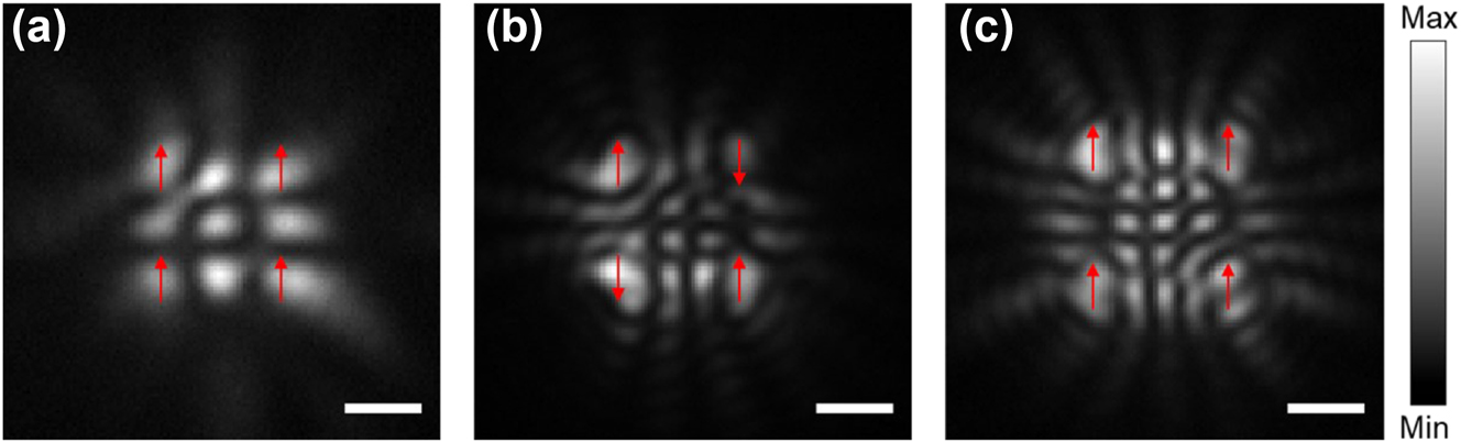
Construction of the two-dimensional polariton spin lattices. (a–c) The time-integrated real-space images of the 2 × 2 polariton condensate square lattices. With increasing lattice distance, the condensate lattices undergo a transition from ferromagnetic to antiferromagnetic and then to the next ferromagnetic coupling states in (a)–(c), respectively. The red arrows marked at the condensates represent the relative spin directions. Scale bars in (a)–(c): 2 μm.

2.4 Theoretical background

We model the lattice of polariton condensates as the system of coupled oscillators [25]

where Ψ i = ρ i exp i θ i is the complex amplitude of the ith oscillator, ρ _i (θ _i ) is its number density (phase), γ inj t is the incoherent injection/gain (assumed uniform for all oscillators), γ _c represents the linear losses, U is polariton–polariton interaction strength, and J _ij is the coupling strength between ith and jth oscillator. We write Eq. (2) as dimensionless; the exact nondimensionalization as well as the approximations used in deriving Eq. (2) can be found in [25]. The coupling strength depends on the number of parameters: shape of the excitation/injection, its intensity, and the distance d _ij between the pumping sites [26]. The first two parameters determine the in-plane momentum of the condensates k _c and the coupling strength varies as a Bessel function of the first kind J i j ≈ J 0 k c d i j taking positive (ferromagnetic coupling) and negative (antiferromagnetic coupling) values [23], [26], [27]. We demonstrate this experimentally by increasing the separation between two condensates (a polariton dyad [28]) and observing the ferromagnetic (in-phase) and antiferromagnetic (antiphase) couplings shown in Figure 3.

The system of Eq. (2) is obtained from the mean-field Ginzburg–Landau equations [29] governing the evolution of the condensates in the lattice using tight-binding approximation integrating over spatial degrees of freedom [25]. The real terms of this equation represent the gradient descent of the loss function F _loss for N condensates:

as

while the last conservative term of Eq. (2) contributes to the phase rotation. The oscillator system minimizes the system’s losses via graduate descent while the injection rate γ ^inj acts as the bifurcation (annealing) parameter, taking the system through the Andronov–Hopf bifurcation [30]. The operation of the system can be compared and contrasted with the Coherent Ising Machine [31], [32], [33], [34], [35], [36], [37], which is the real-valued analog of Eq. (2) where the phases are restricted to take values θ _i ∈ {0, π} and U = 0. When the injection rate (laser power) is small, so γ inj t − γ c < 0 the loss function landscape is convex, with the only minimum occurring at Ψ _i = 0 for all i. As γ inj t increases, the loss landscape will become nonconvex when the complex Hessian matrix with components H Ψ i j = δ 2 F loss δ Ψ j δ Ψ i * acquires a negative eigenvalue. We can bound the minimum eigenvalue λ min H Ψ of H, by Jensen’s inequality

Therefore, λ min H Ψ < 0 (and F _loss can become non-convex) when γ inj > γ c − λ max J ≡ Γ J . As γ ^inj increases, the loss landscape becomes nonconvex and new minima appear along the direction defined by the eigenvector associated with the largest eigenvalue of the coupling matrix J. As the injection increases further, the minima deviate from those defined by the spectral (linear) problem toward the true global minimum of the loss function. With the further injection increase γ inj t ≫ Γ J , the densities tend to minimize the first term of Eq. (3) and reach ρ _i = γ ^inj − γ _c to the leading order while the phases minimize the classical XY Hamiltonian H X Y = − ∑ i , j J i j ⁡ cos θ i − θ j . However, in this case, minimization of H _XY becomes a weak perturbation of the uncoupled system of oscillators. In an analogy with the soft-spin Ising Hamiltonian [38], we refer to F _loss defined in Eq. (3) as “soft-spin” and to H _XY as “hard-spin” XY Hamiltonians.

Finally, more information about the dynamics can be gathered by separating real and imaginary parts of Eq. (2):

The fixed point of Eq. (6) at a particular saturation value of γ ^inj yields

while Eq. (7) represents the Kuramoto oscillators with self-frequencies Uρ _i ; however, the coupling strengths between the Kuramoto oscillators are modified by their amplitudes. A constant relative phase between them will be achieved only if amplitudes are not vastly different.

To summarize, our analysis indicates that as γ ^inj increases, the system undergoes several transitions and for each fixed value of γ ^inj solves a different problem. Close to the condensation threshold when γ inj ≈ Γ J , the system evolves from Ψ _i = 0 state into the state along the negative curvature direction dictated by the principle eigenvector of the coupling matrix J; however, it stabilizes to a fixed point in relative phases only at a higher γ ^inj when amplitudes are sufficiently homogeneous. This fixed point corresponds to the minimum of the loss function, which is a soft-spin version of the classical XY Hamiltonian. In the high injection limit, γ inj ≫ Γ J , the spin densities approach γ ^inj − γ _c with the relative phases reaching a fixed point corresponding to the minimum of the hard-spin XY Hamiltonian. However, the minimization comes as a perturbation. In our experiments, therefore, we do not reach the high intensity limit and observe the minimization of the soft-spin XY Hamiltonian represented by the loss function given by Eq. (3). The density heterogeneities are clearly observed on Figure 4.

To illustrate the evolution and the steady state of our system, we solved the system of Eq. (2) starting with random initial conditions with J ₁₂ = J ₂₃ = J ₃₄ = J ₁₄ = 1 ferromagnetic (F) and J ₁₂ = J ₂₃ = J ₃₄ = J ₁₄ = −1 antiferromagnetic (AF) interactions along the sides of the square formed by four condensates. Without loss of generality, we took U = 1, γ inj t = 10 ⁡ tanh t / 100 + 10 , γ _c = 5. Figure 5 depicts the time evolution of the phases via cos θ i − θ 1 (main panels) and the squares of the complex amplitudes Ψ i 2 (insets) for F (Figure 5(a)) and AF (Figure 5(b)) interactions. As the amplitudes bifurcate from the vacuum states, the phases take the values that minimize the XY Hamiltonian: {0, 0, 0, 0} for F and {0, π, 0, π} for AF interactions. For such simple configuration, the minima of the soft-spin and hard-spin Hamiltonians coincide since the amplitudes take the same values for large times. To see the realization of the soft-spin XY Hamiltonian, we will assume that one of the oscillators is located near a defect and the linear losses for that condensate differ from the rest of the system. Without loss of generality, we will assume that the linear losses are 20 % higher for that condensate, say the condensate Ψ₁. Figure 5(c) shows the time evolution of the phases and the densities of the condensates for AF interactions. The density of the Ψ₁ condensate is depleted with respect to the densities of the other condensates, while the phases deviate from {0, π, 0, π} by δθ ₁ and δθ ₂ and become {0, π + δθ ₁, δθ ₂, π + δθ ₁}, as seen in Figure 5(c). However, configurations with ± δθ ₁ and ± δθ ₂ are equally likely to be realized, so on the time-averaged experiments, like ours, the state {0, π, 0, π} is seen.

Figure 5:

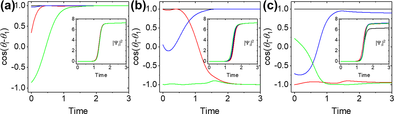
The time evolution of the phases and the squares of the complex amplitudes of four condensates. (a–c) The phases of the condensates represented by cos θ i − θ 1 obtained by numerical integration of the system of Eq. (2) starting with random initial conditions with J ₁₂ = J ₂₃ = J ₃₄ = J ₁₄ = 1 (a) and J ₁₂ = J ₂₃ = J ₃₄ = J ₁₄ = −1 (b, c) interactions along the sides of the square formed by four condensates. Here U = 1 , γ inj t = 10 ⁡ tanh t / 100 + 10 , γ c = 5 . The insets depict the squares of the complex amplitudes Ψ i 2 . The solid lines in black, red, blue, and green represent the phase and the square of the amplitude of the condensates with i = 1 ∼ 4, respectively. (c) The same as (b) but the linear losses are γ _c1 = 1.2γ _ci , i ≠ 1. The single shot experiment phase deviations discussed in the main text are δθ ₁ = ±0.110π, δθ ₂ = ±0.154π.

4.1 Cavity fabrication

12.5 pairs of SiO₂/Ta₂O₅ DBR mirror were deposited on six-inch well-clean quartz wafers by electron beam evaporation with an advanced plasma source. A gold pad array of 250 μm side length was deposited on the DBR surface by electron beam evaporation. Then, two of the same DBR wafers were aligned by the gold pads and bonded together in a wafer bonder. The bonded wafers were diced into 2-cm chips. More details can be found in our previous work [14].

4.2 Synthesis of halide perovskites

The perovskites were grown by an inverse-temperature crystallization method [48]. A droplet of precursors (1.6 M 1:1 mixture of MABr and PbBr₂ in N, N-dimethylformamide) was deposited at the edge of the microcavity and filled the entire microcavity through capillary action. Subsequently, the crystals gradually crystallized as the solubility decreased at 80 °C for 24–48 h in a nitrogen-filled glove box. This solution growth method under confinement can yield high-quality, large-sized perovskite single crystals. After the crystal growth, the cavity with crystals was put in a vacuum chamber at an 80 °C hotplate to remove the residual solvent.

4.3 Optical measurements of polariton

A home-built optical setup in a transmission configuration was used for all the optical measurements. A 450-nm, 250-fs optical parametric amplifier pulsed laser with a 2 kHz repetition rate was used to pump the sample nonresonantly. A phase-only reflective liquid-crystal spatial light modulator was used to generate pumping laser patterns by holograms computed by a Gerchberg–Saxton algorithm. The laser pattern was transferred to an objective (Nikon 40× Plan Fluor ELWD, N.A. = 0.6) with a Fourier imaging configuration. The PL was collected in a transmission configuration with another objective (Nikon 40/60× Plan Fluor ELWD, N.A. = 0.6/0.7). The angle-resolved dispersions were measured by a Fourier imaging system with two achromatic tube lenses and an Andor spectrometer equipped with a two-dimensional CCD. The real-space images were obtained by a two-dimensional Princeton instrument EMCCD.

References

[1] H. Deng, G. Weihs, C. Santori, J. Bloch, and Y. Yamamoto, “Condensation of semiconductor microcavity exciton polaritons,” Science, vol. 298, no. 5591, pp. 199–202, 2002. https://doi.org/10.1126/science.1074464.Search in Google Scholar PubMed
[2] J. Kasprzak, et al.., “Bose-Einstein condensation of exciton polaritons,” Nature, vol. 443, no. 7110, pp. 409–414, 2006. https://doi.org/10.1038/nature05131.Search in Google Scholar PubMed
[3] H. Deng, H. Haug, and Y. Yamamoto, “Exciton-polariton bose-einstein condensation,” Rev. Mod. Phys., vol. 82, no. 2, pp. 1489–1537, 2010. https://doi.org/10.1103/RevModPhys.82.1489.Search in Google Scholar
[4] A. Amo, et al.., “Superfluidity of polaritons in semiconductor microcavities,” Nat. Phys., vol. 5, no. 11, pp. 805–810, 2009. https://doi.org/10.1038/nphys1364.Search in Google Scholar
[5] A. Amo, et al.., “Polariton superfluids reveal quantum hydrodynamic solitons,” Science, vol. 332, no. 6034, pp. 1167–1170, 2011. https://doi.org/10.1126/science.1202307.Search in Google Scholar PubMed
[6] N. G. Berloff, et al.., “Realizing the classical XY Hamiltonian in polariton simulators,” Nat. Mater., vol. 16, no. 11, pp. 1120–1126, 2017. https://doi.org/10.1038/NMAT4971.Search in Google Scholar
[7] Q. Zhang, R. Su, X. Liu, J. Xing, T. C. Sum, and Q. Xiong, “High-quality whispering-gallery-mode lasing from cesium lead halide perovskite nanoplatelets,” Adv. Funct. Mater., vol. 26, no. 34, pp. 6238–6245, 2016. https://doi.org/10.1002/adfm.201601690.Search in Google Scholar
[8] J. V. Passarelli, et al.., “Tunable exciton binding energy in 2D hybrid layered perovskites through donor–acceptor interactions within the organic layer,” Nat. Chem., vol. 12, no. 8, pp. 672–682, 2020. https://doi.org/10.1038/s41557-020-0488-2.Search in Google Scholar PubMed
[9] S. D. Stranks and H. J. Snaith, “Metal-halide perovskites for photovoltaic and light-emitting devices,” Nat. Nanotechnol., vol. 10, no. 5, pp. 391–402, 2015. https://doi.org/10.1038/nnano.2015.90.Search in Google Scholar PubMed
[10] A. Fieramosca, et al.., “Two-dimensional hybrid perovskites sustaining strong polariton interactions at room temperature,” Sci. Adv., vol. 5, no. 5, p. eaav9967, 2019. https://doi.org/10.1126/sciadv.aav9967.Search in Google Scholar PubMed PubMed Central
[11] R. Su, et al.., “Room-temperature polariton lasing in all-inorganic perovskite nanoplatelets,” Nano Lett., vol. 17, no. 6, pp. 3982–3988, 2017. https://doi.org/10.1021/acs.nanolett.7b01956.Search in Google Scholar PubMed
[12] R. Su, et al.., “Observation of exciton polariton condensation in a perovskite lattice at room temperature,” Nat. Phys., vol. 16, no. 3, pp. 301–306, 2020. https://doi.org/10.1038/s41567-019-0764-5.Search in Google Scholar
[13] K. Peng, et al.., “Room-temperature polariton quantum fluids in halide perovskites,” Nat. Commun., vol. 13, no. 1, p. 7388, 2022. https://doi.org/10.1038/s41467-022-34987-y.Search in Google Scholar PubMed PubMed Central
[14] R. Tao, et al.., “Halide perovskites enable polaritonic XY spin Hamiltonian at room temperature,” Nat. Mater., vol. 21, no. 7, pp. 761–766, 2022. https://doi.org/10.1038/s41563-022-01276-4.Search in Google Scholar PubMed
[15] H. Zhou, et al.., “Interface engineering of highly efficient perovskite solar cells,” Science, vol. 345, no. 6196, pp. 542–546, 2014. https://doi.org/10.1126/science.1254050.Search in Google Scholar PubMed
[16] L. Polimeno, et al.., “Observation of two thresholds leading to polariton condensation in 2D hybrid perovskites,” Adv. Opt. Mater., vol. 8, no. 16, p. 2000176, 2020. https://doi.org/10.1002/adom.202000176.Search in Google Scholar
[17] K. Galkowski, et al.., “Determination of the exciton binding energy and effective masses for methylammonium and formamidinium lead tri-halide perovskite semiconductors,” Energy Environ. Sci., vol. 9, no. 3, pp. 962–970, 2016. https://doi.org/10.1039/c5ee03435c.Search in Google Scholar
[18] Y. Yang, M. Yang, Z. Li, R. Crisp, K. Zhu, and M. C. Beard, “Comparison of recombination dynamics in CH3NH3PbBr3 and CH3NH3PbI3 perovskite films: influence of exciton binding energy,” J. Phys. Chem. Lett., vol. 6, no. 23, pp. 4688–4692, 2015. https://doi.org/10.1021/acs.jpclett.5b02290.Search in Google Scholar PubMed
[19] F. Ruf, et al.., “Temperature-dependent studies of exciton binding energy and phase-transition suppression in (Cs,FA,MA)Pb(I,Br)3 perovskites,” APL Mater., vol. 7, no. 3, p. 31113, 2019. https://doi.org/10.1063/1.5083792.Search in Google Scholar
[20] R. J. Elliott, “Intensity of optical absorption by excitons,” Phys. Rev., vol. 108, no. 6, pp. 1384–1389, 1957. https://doi.org/10.1103/PhysRev.108.1384.Search in Google Scholar
[21] M. Saba, et al.., “Correlated electron–hole plasma in organometal perovskites,” Nat. Commun., vol. 5, no. 1, p. 5049, 2014. https://doi.org/10.1038/ncomms6049.Search in Google Scholar PubMed
[22] M. Wouters, I. Carusotto, and C. Ciuti, “Spatial and spectral shape of inhomogeneous nonequilibrium exciton-polariton condensates,” Phys. Rev. B, vol. 77, no. 11, p. 115340, 2008. https://doi.org/10.1103/PhysRevB.77.115340.Search in Google Scholar
[23] H. Ohadi, et al.., “Nontrivial phase coupling in polariton multiplets,” Phys. Rev. X, vol. 6, no. 3, p. 031032, 2016. https://doi.org/10.1103/PhysRevX.6.031032.Search in Google Scholar
[24] G. Tosi, et al.., “Geometrically locked vortex lattices in semiconductor quantum fluids,” Nat. Commun., vol. 3, no. 1, p. 1243, 2012. https://doi.org/10.1038/ncomms2255.Search in Google Scholar PubMed
[25] K. P. Kalinin and N. G. Berloff, “Polaritonic network as a paradigm for dynamics of coupled oscillators,” Phys. Rev. B, vol. 100, no. 24, p. 245306, 2019. https://doi.org/10.1103/PhysRevB.100.245306.Search in Google Scholar
[26] P. G. Lagoudakis and N. G. Berloff, “A polariton graph simulator,” New J. Phys., vol. 19, no. 12, p. 125008, 2017. https://doi.org/10.1088/1367-2630/aa924b.Search in Google Scholar
[27] K. P. Kalinin and N. G. Berloff, “Networks of non-equilibrium condensates for global optimization,” New J. Phys., vol. 20, no. 11, p. 113023, 2018. https://doi.org/10.1088/1367-2630/aae8ae.Search in Google Scholar
[28] A. Johnston, K. P. Kalinin, and N. G. Berloff, “Artificial polariton molecules,” Phys. Rev. B, vol. 103, no. 6, p. L060507, 2021. https://doi.org/10.1103/PhysRevB.103.L060507.Search in Google Scholar
[29] J. Keeling and N. G. Berloff, “Spontaneous rotating vortex lattices in a pumped decaying condensate,” Phys. Rev. Lett., vol. 100, no. 25, p. 250401, 2008. https://doi.org/10.1103/PhysRevLett.100.250401.Search in Google Scholar PubMed
[30] M. Syed and N. G. Berloff, “Physics-enhanced bifurcation optimisers: all you need is a canonical complex network,” IEEE J. Sel. Top. Quantum Electron., vol. 29, no. 2, pp. 1–6, 2023. https://doi.org/10.1109/JSTQE.2023.3235334.Search in Google Scholar
[31] T. Inagaki, et al.., “A coherent Ising machine for 2000-node optimization problems,” Science, vol. 354, no. 6312, pp. 603–606, 2016. https://doi.org/10.1126/science.aah4243.Search in Google Scholar PubMed
[32] A. Yamamura, K. Aihara, and Y. Yamamoto, “Quantum model for coherent Ising machines: discrete-time measurement feedback formulation,” Phys. Rev. A, vol. 96, no. 5, p. 53834, 2017. https://doi.org/10.1103/PhysRevA.96.053834.Search in Google Scholar
[33] M. Calvanese Strinati, D. Pierangeli, and C. Conti, “All-optical scalable spatial coherent ising machine,” Phys. Rev. Appl., vol. 16, no. 5, p. 54022, 2021. https://doi.org/10.1103/PhysRevApplied.16.054022.Search in Google Scholar
[34] P. L. McMahon, et al.., “A fully programmable 100-spin coherent Ising machine with all-to-all connections,” Science, vol. 354, no. 6312, pp. 614–617, 2016. https://doi.org/10.1126/science.aah5178.Search in Google Scholar PubMed
[35] Y. Yamamoto, T. Leleu, S. Ganguli, and H. Mabuchi, “Coherent Ising machines—quantum optics and neural network Perspectives,” Appl. Phys. Lett., vol. 117, no. 16, p. 160501, 2020. https://doi.org/10.1063/5.0016140.Search in Google Scholar
[36] Y. Yamamoto, et al.., “Coherent Ising machines—optical neural networks operating at the quantum limit,” NPJ Quantum Inf., vol. 3, no. 1, p. 49, 2017. https://doi.org/10.1038/s41534-017-0048-9.Search in Google Scholar
[37] Z. Wang, A. Marandi, K. Wen, R. L. Byer, and Y. Yamamoto, “Coherent Ising machine based on degenerate optical parametric oscillators,” Phys. Rev. A, vol. 88, no. 6, p. 63853, 2013. https://doi.org/10.1103/PhysRevA.88.063853.Search in Google Scholar
[38] H. Sompolinsky and A. Zippelius, “Relaxational dynamics of the Edwards-Anderson model and the mean-field theory of spin-glasses,” Phys. Rev. B, vol. 25, no. 11, pp. 6860–6875, 1982. https://doi.org/10.1103/PhysRevB.25.6860.Search in Google Scholar
[39] D. Ballarini, et al.., “Polaritonic neuromorphic computing outperforms linear classifiers,” Nano Lett., vol. 20, no. 5, pp. 3506–3512, 2020. https://doi.org/10.1021/acs.nanolett.0c00435.Search in Google Scholar PubMed
[40] N. Stroev and N. G. Berloff, “Neural network architectures based on the classical XY model,” Phys. Rev. B, vol. 104, no. 20, p. 205435, 2021. https://doi.org/10.1103/PhysRevB.104.205435.Search in Google Scholar
[41] K. P. Kalinin and N. G. Berloff, “Large-scale sustainable search on unconventional computing hardware,” 2021, arXiv Prepr. arXiv2104.02553.Search in Google Scholar
[42] N. Stroev and N. G. Berloff, “Analog photonics computing for information processing, inference, and optimization,” Adv. Quantum Technol., vol. 6, no. 9, p. 2300055, 2023. https://doi.org/10.1002/qute.202300055.Search in Google Scholar
[43] S. Alyatkin, J. D. Töpfer, A. Askitopoulos, H. Sigurdsson, and P. G. Lagoudakis, “Optical control of couplings in polariton condensate lattices,” Phys. Rev. Lett., vol. 124, no. 20, p. 207402, 2020. https://doi.org/10.1103/PhysRevLett.124.207402.Search in Google Scholar PubMed
[44] J. D. Töpfer, I. Chatzopoulos, H. Sigurdsson, T. Cookson, Y. G. Rubo, and P. G. Lagoudakis, “Engineering spatial coherence in lattices of polariton condensates,” Optica, vol. 8, no. 1, pp. 106–113, 2021. https://doi.org/10.1364/optica.409976.Search in Google Scholar
[45] M. Furman, et al.., “Magneto-optical induced supermode switching in quantum fluids of light,” Commun. Phys., vol. 6, no. 1, p. 196, 2023. https://doi.org/10.1038/s42005-023-01319-5.Search in Google Scholar
[46] T. Wang, et al.., “Electrically pumped polarized exciton-polaritons in a halide perovskite microcavity,” Nano Lett., vol. 22, no. 13, pp. 5175–5181, 2022. https://doi.org/10.1021/acs.nanolett.2c00906.Search in Google Scholar PubMed
[47] H. Kang, J. Ma, J. Li, X. Zhang, and X. Liu, “Exciton polaritons in emergent two-dimensional semiconductors,” ACS Nano, vol. 17, no. 24, pp. 24449–24467, 2023. https://doi.org/10.1021/acsnano.3c07993.Search in Google Scholar PubMed
[48] X. D. Wang, W. G. Li, J. F. Liao, and D. Bin Kuang, “Recent advances in halide perovskite single-crystal thin films: fabrication methods and optoelectronic applications,” Sol. RRL, vol. 3, no. 4, p. 1800294, 2019. https://doi.org/10.1002/SOLR.201800294.Search in Google Scholar
© 2024 the author(s), published by De Gruyter, Berlin/Boston
This work is licensed under the Creative Commons Attribution 4.0 International License.
Articles in the same Issue
- Frontmatter
- Editorial
- Strong Coupling of Organic Molecules 2023 (SCOM23)
- Perspective
- Strong coupling of metamaterials with cavity photons: toward non-Hermitian optics
- Research Articles
- Strong coupling in molecular systems: a simple predictor employing routine optical measurements
- Extracting accurate light–matter couplings from disordered polaritons
- Linear optical properties of organic microcavity polaritons with non-Markovian quantum state diffusion
- Non-Hermitian polariton–photon coupling in a perovskite open microcavity
- Realization of ultrastrong coupling between LSPR and Fabry–Pérot mode via self-assembly of Au-NPs on p-NiO/Au film
- Self-hybridisation between interband transitions and Mie modes in dielectric nanoparticles
- Probing the anharmonicity of vibrational polaritons with double-quantum two-dimensional infrared spectroscopy
- Enhancement of the internal quantum efficiency in strongly coupled P3HT-C60 organic photovoltaic cells using Fabry–Perot cavities with varied cavity confinement
- Active control of polariton-enabled long-range energy transfer
- Coherent transient exciton transport in disordered polaritonic wires
- Identifying the origin of delayed electroluminescence in a polariton organic light-emitting diode
- Extracting kinetic information from short-time trajectories: relaxation and disorder of lossy cavity polaritons
- Exploring the impact of vibrational cavity coupling strength on ultrafast CN + c-C6H12 reaction dynamics
- Resonance theory of vibrational polariton chemistry at the normal incidence
- Investigating the collective nature of cavity-modified chemical kinetics under vibrational strong coupling
- Thermalization rate of polaritons in strongly-coupled molecular systems