Describing the Pearson 𝑅 distribution of aggregate data

2.1 Sampling from a bivariate distribution

If one samples {(xi,yi), 1≤i≤n} from a bivariate distribution

where ρ is the level of correlation, μx and μy are the x-mean and y-mean, and σx and σy are the standard deviation for x and y, respectively, the sample Pearson R coefficient

will have the distribution

where Γ is the gamma function and F12 is the generalized hypergeometric function [10]. The distribution (2.2) can be constructed using the series provided by [10]

Moreover, the estimate provided by the sample is biased and underestimates ρ. The expectation E⁡(R) and the variance Var⁡(R) are provided by Muirhead [10],

where O⁢(n-2) refers to omitted terms on the order of 1np, where p≥2. Thus the difference between ρ and E⁡(R) can be estimated to first order using

The distribution (2.2) is not symmetric. However, Fisher [2] proposed the transformation

and it can be shown [10] that the resulting distribution approaches a normal distribution with standard deviation

as n→∞. Table 1 reports the ratio of the standard deviation σz to the standard deviation of the distribution (2.2) after Fisher’s transformation is applied for two values of ρ=0 and ρ=0.7. The ratio rapidly approaches 1.0 as n increases.

2.2 Bivariate distribution of averages

The distribution of averages sampled from a bivariate distribution (2.1)

is described by [3] as

where xi(k) and yi(k) refer to the i-th member of the k-th group and ℬ is the bivariate distribution defined in equation (2.1). While the standard deviations are different in the arguments of (2.1) and (2.7), the Pearson R distribution (2.2) does not depend on the standard deviations. Therefore, the distribution (2.2) also applies to averages (x¯k,y¯k).

Figure 1

The analytical distribution (2.2) accurately represents the distribution created by n groups, where each of the n groups is formed by averaging m scores sampled from a bivariate distribution with ρ=0.7. In the figure, n=512m. For each value of m, 100,000 different random samples of size n⋅m=512 were chosen, and therefore 100,000 R values based on the averages were used to form each of the distributions shown as “bivariate avg” in the figure.

Figure 1 confirms this with a Monte Carlo simulation and random sampling for ρ=0.7. If n groups of m scores are drawn from a bivariate distribution and the groups of m scores are averaged, the distribution of the Pearson R based on the averaged scores matches the distribution (2.2) which is generated using (2.3). In Figure 1, n=512m groups are formed, where each group has m scores sampled from the bivariate distribution (2.1). The values of m used are m=2,4,8,16,32,64, and 128. The number of samples of size n⋅m=512 used to create each distribution for each value of m is 100,000. Sampling is done by first finding each xi(k) and yi(k)⁣* by randomly sampling from a normal distribution with a mean of zero and a standard deviation of one. The scores are then correlated using

3.1 Defining a partition

We now describe the distribution of Pearson R coefficients created from group averages formed from a fixed sample of scores of length n. This requires us to define a partition of a set of original scores, where the scores are divided into subsets of equal size m.

Given a set of original scores X={xi, 1≤i≤n}, Y={yi, 1≤i≤n}, define a set Pk to be a group of m indices, where m<n and n is divisible by m,

where each index 1≤ijk≤n is unique (i.e. ij1k≠ij2k when j1≠j2). Construct all the nm sets Pk so that they are disjoint,

and so the union of all the Pk sets forms the entire set of integers ranging from 1 to n. We refer to the collection of all Pk sets as a partition

There exist

groups Pk in the partition P. For each Pk in the partition P, construct the mean scores

Assemble all the pairs {(x¯k,y¯k),k=1,2,…,nm}, and define Rx¯,y¯ to be the Pearson correlation coefficient computed from these pairs,

Let us illustrate the process with an actual example. Suppose we have the following n=8 elements in sets X and Y: X={x1,x2,x3,x4,x5,x6,x7,x8} and Y={y1,y2,y3,y4,y5,y6,y7,y8}. Using a group size of m=2, one can select the sets P1={1,5}, P2={2,4}, P3={3,7} and P4={6,8}. This selection of Pk’s divides the 8 original elements in X and Y into nm=4 groups

The average x¯k values are x¯1=(x1+x5)/2, x¯2=(x2+x4)/2, x¯3=(x3+x7)/2 and x¯4=(x6+x8)/2. The corresponding average y¯k values are also computed. The Pearson Rx¯,y¯ value is then computed from these average pairs {(x¯1,y¯1),(x¯2,y¯2),(x¯3,y¯3),(x¯4,y¯4)} using (3.2).

The number of partitions that can be constructed using groups of size m from n individual scores is

The expression in (3.3) is derived by first choosing m elements from n elements, (nm). Given the remaining n-m elements, there are (n-mm) ways of choosing the second group of m elements. Continuing, there are

number of ways of choosing all groups. However, since order does not matter when choosing a partition, equation (3.4) needs to be divided by the number of ways of reordering the groups (i.e. nm!) which yields (3.3).

Figure 2 shows the number of partitions for different group sizes m for n=120 original scores. The vertical axis uses a log scale because of the wide range of scores. For example, 80 on the vertical axis corresponds to 1080 partitions.

Figure 2

log10 of the number of partitions (3.3) for n=120 original scores and different group sizes m.

3.2 Constructing the Pearson Rx¯,y¯ distribution with simulations

Section 2.2 showed that the Pearson R coefficient generated from averaged data sampled from a bivariate distribution follows the distribution described by equation (2.2). In contrast, to create the Pearson R distribution from a partition, a set of n individual scores is chosen and remains fixed. Each partition rearranges the n original scores into nm different groups each of size m. A Pearson Rx¯,y¯ value is generated based on the nm average scores.

Constructing the exact distribution using partitions would require one to compute the fraction of all possible partitions that produce a Pearson Rx¯,y¯ coefficient that resides within a series of intervals that fill the range between -1 and 1. We do not attempt to develop the theory that underlies the exact distribution but instead rely on a series of Monte Carlo simulations to describe the distribution of Pearson Rx¯,y¯ coefficients. Our Monte Carlo simulations show that the Pearson Rx¯,y¯ values generated from the randomly generated partitions are similar to the distribution described by (2.2). However, there are differences for small group sizes, which diminish as the group size m increases. The symbols we use in our simulations are summarized in Table 2. We refer to the distribution of Rx¯,y¯ values created from the randomly generated partitions as the partition distribution.

We begin by generating the scores

where each xi and yi* is randomly sampled from a normal distribution with a mean of zero and a standard deviation of one. The scores are then correlated using the equivalent of equation (2.8)

In Figure 3, we sample 1,000 different sets of n=64 individual scores from a bivariate distribution (2.1) with ρ=0.7 using (3.6). An Rindividual value is computed for each of the 1,000 different samples and plotted on the horizontal axis. For each of the 1,000 samples, 10,000 different partitions and their corresponding Rx¯,y¯ values are generated with group size m=4. The average Pearson value R¯x¯,y¯ is computed by averaging the 10,000 Rx¯,y¯ values from each partition distribution thus forming an approximation to the expected value for the distribution. The difference between Rindividual and R¯x¯,y¯ is plotted on the vertical axis. Figure 3 shows that the expected value R¯x¯,y¯ underpredicts Rindividual since the differences are all positive. Therefore, according to these simulations, the expected value from the partition distribution is a biased estimate of Rindividual at least for finite n. The difference Rindividual-R¯x¯,y¯ also appears to decrease as Rindividual increases.

Figure 3

Difference between Rindividual and the expected value R¯x¯,y¯ generated by averaging 10,000 Rx¯,y¯ values corresponding to 10,000 partitions with group size m=4 generated from each of the 1,000 different samples of length n=64 drawn from a bivariate distribution. Each partition contained nm=16 groups. The original scores were generated by sampling from a bivariate distribution with ρ=0.7 using equations (3.5) and (3.6). R¯x¯,y¯ underpredicts Rindividual in all 1,000 cases although all errors are less than 0.0017.

Figure 4

Difference between Rindividual and R¯x¯,y¯ generated from 100 different samples as a function of the number of groups nm. All samples are drawn from a bivariate normal distribution with ρ=0.7. For each sample, 10,000 partitions are generated. The 10,000 Rx¯,y¯ values generated for each partition are averaged to form the expected value R¯x¯,y¯. The 100 differences Rindividual-R¯x¯,y¯ are averaged again and plotted. Equation (3.7) plotted in yellow estimates the difference Rindividual-R¯x¯,y¯ well for a large number of groups nm.

Figure 5

Difference in maximum and minimum value R¯x¯,y¯ generated from 100 different samples. All samples are drawn from a bivariate normal distribution with ρ=0.7. For each sample, 10,000 partitions are generated. The 10,000 Rx¯,y¯ values generated for each partition are averaged to form the expected value R¯x¯,y¯. The maximum and minimum of the 100 values of R¯x¯,y¯ are then found and the difference is plotted. The difference decreases as the number of groups nm increases.

To address the impact a specific individual sample has on the set of Rx¯,y¯ coefficients and the average R¯x¯,y¯ value, we generate 100 different samples from a bivariate distribution with ρ=0.7 using (3.5) and (3.6). For consistency, equations (3.5) and (3.6) are now solved repeatedly until Rindividual and ρ=0.7 agree to within 0.0001 before an individual sample is selected to be one of the 100 samples. The solving of (3.5) and (3.6) repeatedly until Rindividual and ρ agree to within 0.0001 is also used in the remaining figures with the exception of Figures 15 and 17. For each sample, 10,000 different partitions are generated, and Rx¯,y¯ is generated for each partition. The 10,000 values of Rx¯,y¯ are then averaged to form R¯x¯,y¯. Figure 4 plots the average difference Rindividual-R¯x¯,y¯ of the 100 different samples as a function of the number of groups nm. Different sample sizes n and group sizes m are used: n=210, m=2,3,5,7,10,15,21; n=512, m=2,4,8,16,32,64,128; n=1,024, m=8,16,32,64,128,256; n=2,048, m=32,64,128,256; n=4,096, m=256. The logarithm log2⁡(nm) is used along the horizontal axis to compress the horizontal range. Figure 4 shows that the expected R¯x¯,y¯ value is a biased estimate and underestimates Rindividual. However, the graph also shows that, as the number of groups nm in the partition increases, the average error and error bar range decrease. An error estimate E⁡(Rindividual,nm) shown in equation (3.7) is also plotted in yellow for comparison. The equation shows that E⁡(Rindividual,nm) estimates the first-order error Rindividual-R¯x¯,y¯ well for a number of groups nm>8,

Equation (3.7) is generated by replacing ρ with Rindividual and n with nm in equation (2.4). The difference between the maximum R¯x¯,y¯ and minimum R¯x¯,y¯ over the 100 samples is plotted in Figure 5. The difference decreases as the number of groups increases.

Figure 6 compares the analytical distribution

to the partition distribution formed by randomly generating 50,000 partitions for n=512 scores sampled from the bivariate distribution and different group sizes, m=2,4,8,16,32,64 and 128 corresponding to the number of groups nm=256,128,64,32,16,8 and 4. The analytical distribution (3.8) is essentially (2.2) with R, ρ and n replaced with Rx¯,y¯, Rindividual and nm, respectively. Higher peaks are clearly evident for group sizes m=2 and m=4 for the partition distribution labelled “partition” compared to the analytical distribution. The partition distributions for group sizes m=2 and m=4 also have smaller standard deviations compared to the analytical distribution (3.8). This trend is present for the same simulation performed with ρ=0 shown in Figure 7. For larger group sizes (m>8), the partition distribution agrees well with the analytical distribution. Differences between (3.8) and the partition distribution for ρ=0.7 are shown in Figure 8.

Figure 6

Comparing the analytical distribution (3.8) to the partition distribution for n=512, ρ=0.7 and different group sizes m. The number of groups nm is nm. The 512 scores are sampled from a bivariate distribution. For each group size, 50,000 partitions were used to create the partition distribution.

Figure 7

Comparing the analytical distribution (3.8) to the partition distribution for n=512, ρ=0 and different group sizes m. The number of groups nm is nm. The 512 scores are sampled from a bivariate distribution. For each group size, 50,000 partitions were used to create the partition distribution.

Figure 8

Difference between analytical distribution (3.8) and partition distribution for n=512, ρ=0.7 and different group sizes m. The number of groups nm is nm. The 512 scores are sampled from a bivariate distribution. The difference decreases as the group size m increases. For each group size, 50,000 partitions were used to create the partition distribution.

We also create the partition distribution for scores randomly sampled from a uniform distribution, 0≤xi≤1, 0≤yi≤1, and correlated using (3.6) with ρ=0.7. For each different group size, 50,000 partitions are generated. Differences between (3.8) and the partition distribution are shown in Figure 9. The high degree of similarity between Figures 8 and 9 shows that sampling from either a bivariate or uniform distribution does not affect the partition distributions.

Figure 9

Difference between analytical distribution (3.8) and partition distribution for n=512, ρ=0.7 and different group sizes m. The number of groups nm is nm. The 512 scores are sampled from a uniform distribution. The difference decreases as the group size m increases. For each group size, 50,000 partitions were used to create the partition distribution.

Figure 10 uses different group sizes m=2,4,8 and 64 and a fixed number of groups nm=16. For each group size, 50,000 partitions are generated. Samples are drawn from a bivariate distribution with ρ=0.7. We see that, as the group size increases, the partition distributions converge to the analytical distribution (3.8). Figure 11 compares the analytical distribution described by (3.8) to the partition distribution formed by randomly generating 50,000 partitions for n=512 scores sampled from a bivariate distribution with group size m=16 and number of groups nm=32 for different values of ρ=-0.7,-0.5,-0.2,0.1,0.4 and 0.8. The partition distribution agrees with the analytical distribution for all values of ρ.

Figure 10

Comparing the analytical distribution (3.8) to the partition distribution for number of groups nm=16, ρ=0.7 and different group sizes m. As the group size increases, the partition distributions converge to the analytical distribution. For each group size, 50,000 partitions were used to create the partition distribution. The original scores are sampled from a bivariate distribution.

Figure 11

Comparing the analytical distribution to the partition distribution for different values of ρ, n=512 scores sampled from a bivariate distribution, and m=16. For each value of ρ, 50,000 partitions were used to create the partition distribution.

Figure 12

Comparing the analytical distribution to the partition distribution for different values of ρ for n=512 scores sampled from a bivariate distribution. Sixteen of the groups have size m=16, and eight of the groups have size m=32. The number of groups nm=24. For each value of ρ, 50,000 partitions were used to create the partition distribution.

Figure 12 compares the analytical distribution described by (3.8) to the partition distribution formed by randomly generating 50,000 partitions for n=512 scores sampled from a bivariate distribution and a mixture of group sizes m=16 and m=32 for different values of ρ=-0.7,-0.5,-0.2,0.1,0.4 and 0.8. Sixteen of the groups have size m=16, and eight of the groups have size m=32 in each partition. In the analytical distribution (3.8), we set nm=24 since there are 24 total groups in each partition. We see that the partition distribution agrees well with the analytical distribution for all values of ρ in spite of the fact that the partition is composed of groups of different size.

Figure 13 shows the ratio

of the standard deviation of the analytical distribution sanalytical (3.8) to standard deviation of the partition distribution spartition for ρ=0.7 under the same conditions described in Figure 4. For each value of the sample size n and the group size m, 100 different samples were generated. The analytical distribution has a larger standard deviation than the partition distribution, which is quite evident for smaller group sizes. The logarithm log2⁡(m) is used along the horizontal axis to compress the horizontal range. We see that the standard deviation of the partition distribution approaches the standard deviation of the analytical distribution as the group size increases.

Figure 13

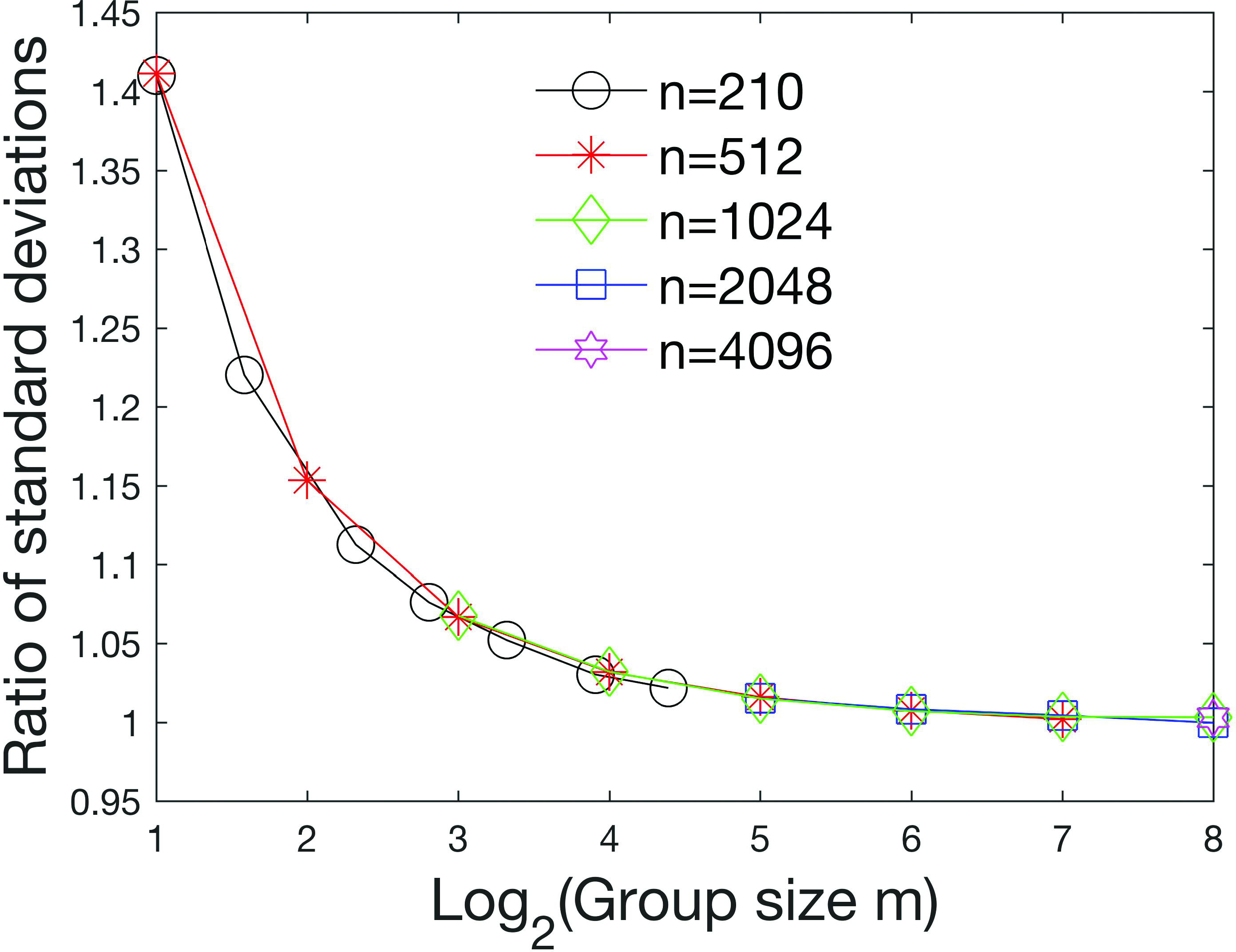
Ratio of standard deviation of analytical distribution to the partition distribution (3.9) for ρ=0.7, sample sizes n=210, n=512, n=1,024, n=2,048 and n=4,096, and different group sizes m. For each value of n and m, 100 different samples are chosen, and 10,000 partitions are created for each sample.

Figure 14

In a follow-up to Figure 13, the difference between maximum and minimum standard deviation ratio (3.9) for all 100 samples for ρ=0.7 and each value of n and m is plotted.

The difference between the maximum ratio and the minimum ratio over all 100 samples for all values of n and m is plotted in Figure 14. For some sample sizes (e.g. n=512, n=2,048), there seems to be a slight increase in the difference as the group size m increases and the corresponding number of groups nm decreases. However, the difference between the maximum ratio and the minimum ratio is less than 0.065 for all values of n and m.

These Monte Carlo simulations suggest that the distribution of Pearson Rx¯,y¯ values can be approximated (for group sizes m>8) with the distribution described by (3.8).

4.1 Confidence intervals for large group sizes m

Since the partition distribution will approach (3.8) as the group size m increases, Fisher’s transformation (2.5) can be used to transform the set of Rx¯,y¯ values to z-values that become normally distributed as nm grows large. Confidence intervals can then be constructed from the normal distribution to predict the individual Pearson R value from the average Pearson Rx¯,y¯ value according to equations (2.5) and (2.6). First the Fisher transformed (see (2.5)) z-value is computed from Rx¯,y¯,

For a C % confidence interval, zα/2 is found, where zα/2 is the z-value above which 12⁢(100-C100) of a standard normal distribution (μ=0,σ=1) area lies,

For example, for a 95 % confidence interval, the value of zα/2 is the z-value above which 0.025 of the standard normal distribution area lies. The lower and upper z-values of the confidence interval are then computed using

where nm is the number of groups used to compute the Rx¯,y¯ value. The values of zl and zu are then transformed back to R values using

to generate the confidence interval (Rl,Ru).

Equations (4.1)–(4.4) can be used to generate confidence intervals (Rl,Ru) for Rindividual given Rx¯,y¯ as long as the group size is large (m>8) and the number of groups nm is large. A large value of nm also reduces the bias according to (3.7). Table 3 show the 95 % confidence intervals (Rl,Ru) for different values of Rx¯,y¯ and different number of groups nm. The confidence interval ranges are narrow for values of Rx¯,y¯ close to 1 and large values of nm. Figure 15 creates a filled contour plot of the 95 % confidence interval width Ru-Rl as a function of Rx¯,y¯ and the number of groups.

Figure 15

Width of confidence interval Ru-Rl for Rindividual as a function of Rx¯,y¯ and the number of groups nm. Narrow widths (represented by darker shades of blue) occur for absolute values of Rx¯,y¯ close to one and for a large number of groups.

4.2 Confidence intervals for small group sizes m≤8

If the group sizes m are not large, the process of generating the confidence intervals shown in equations (4.1)–(4.4) will need to be revised to account for the fact that the analytical distribution has a larger standard deviation compared to the partition distribution. Figure 16 compares the analytical distribution (3.8) to the partition distribution created through Monte Carlo simulation and random sampling after Fisher’s transformation (2.5) is applied for ρ=0.7. Similar to Figure 6, small group sizes (e.g. m=2 and m=4) have a smaller standard deviation compared to the analytical distribution.

Figure 16

Comparing the analytical distribution (3.8) to the partitioning distribution for different group sizes m for ρ=0.7 after Fisher’s transformation (2.5) is applied. Small group sizes m=2 and m=4 have a larger peak and a smaller standard deviation compared to the analytical distribution. For each group size, 50,000 partitions were used to create the partition distribution.

We assess whether the partition distributions for small group sizes m=2, m=4 and m=8 can be approximated by a normal distribution by plotting the Fisher z-values (4.1) arranged in ascending order against the z-values (extracted from a normal distribution) corresponding to a measure fi of the distribution area below each Fisher z-value,

In (4.5), i refers to the location of the Fisher z-value when all the values are arranged in ascending order, and I refers to the total number of values in the distribution. If the plot of the Fisher z-values versus the z-values extracted from the normal distribution is linear, the partition distribution is normal [15]. This plot is shown in Figure 17. Except for extreme z-values, |z|>3.2, which constitute only 0.13 % of all the z-values, the distributions can be approximated by a normal distribution.

Figure 17

The z-values extracted from a normal distribution are plotted against the Fisher z-values for group sizes m=2, m=4 and m=8. The figure shows that, except for extreme z-values |z|>3.2 which constitute only 0.13 % of all the z-values, the distributions can be approximated by a normal distribution. The 30,000 partitions and 30,000 Rx¯,y¯ values are computed for each of the partition distributions which are generated from of sample of length n=1,024 formed using a bivariate distribution with ρ=0.7. The black lines are generated by constructing the least squares line for values of |z|≤3.2.

Figure 18

Ratio of standard deviation of analytical normal distribution (4.6) to the partition distribution for different group sizes m and sample sizes n for ρ=0.7 after Fisher’s transformation is applied. The curve fit function β⁢(m) from equation (4.8) is also plotted.

Figure 19

Ratio of standard deviation of analytical normal distribution (4.6) to the partition distribution for different group sizes m for ρ=0 after Fisher’s transformation is applied. The curve fit function β⁢(m) from equation (4.8) is also plotted.

Figure 18 plots the ratio

of the standard deviation of Fisher’s transformed analytical distribution

to the standard deviation of Fisher’s transformed partition distribution spartitionFisher for ρ=0.7. Different group sizes m are used with a variety of different sampling lengths n=210, n=512, n=1,024, n=2,048 and n=4,096. For each value of n and m, 100 different samples were generated, and 10,000 randomly created partitions were used to create the partition distribution for each of the 100 different samples. Similar to Figure 13, Figure 18 shows that the Fisher transformed analytical distribution has a larger standard deviation than the Fisher transformed partition distribution for small group sizes. The standard deviation of the partition distribution approaches the standard deviation of the analytical distribution as the group size increases. However, to account for the difference in the standard deviations for smaller group sizes, we also fit a curve β⁢(m) to the data to approximate Rsd which is shown in yellow,

Figure 18 only uses combinations of n and m, so the number of groups nm=nm is at least 16 since the number of groups need to be fairly large in order for (4.7) to be valid. Figure 19 performs the same simulation as Figure 18 except ρ=0. (Also, to reduce the computational cost, n=4,096 is not used, and only m=32 is used for n=1,024, and only m=64 is used for n=2,048.) Figure 19 shows that (4.8) is still a good approximation to the ratio of the standard deviations when ρ=0.

Equations (4.1)–(4.4) can still be used to compute the confidence intervals, but equation (4.3) is replaced with

(4.9)

We also increase the standard deviation by 3 % (reflected by the 1.03 in equation (4.9)) to account for the bias (3.7) and the range in standard deviations seen in Figure 14.

4.3 Assessing the accuracy of the confidence intervals

A simulation is performed to assess the accuracy of the confidence intervals computed using (4.9). A value of ρ is selected from ρ=-0.9,-0.5,0,0.3 and 0.7, and a group size is selected from m=2,4,8,16 for nm=32 number of groups. The number of original scores n is n=32⁢m according to (3.1). One hundred samples are generated from a bivariate distribution. Equations (3.5) and (3.6) are repeatedly solved until the difference between Rindividual and ρ is less than 0.0001 for each sample. For each sample, 10,000 different partitions and therefore 10,000 Rx¯,y¯ values are generated. For each Rx¯,y¯ value, a confidence interval is created and the percent Pr of the 10,000 partitions that contain Rindividual is computed. Table 4 shows the minimum percent (Prmin) and maximum percent (Prmax) as a range (Prmin,Prmax) for all 100 samples. Ideally, the ranges should be tightly centered around 95 %. These ranges do confirm that the confidence intervals can be used to approximate the value of Rindividual.

References

[1] G. Firebaugh, A rule for inferring individual-level relationships from aggregate data, Amer. Sociological Rev. 43 (1978), no. 4, 522–557. 10.2307/2094779Search in Google Scholar
[2] R. A. Fisher, On the probable error of a coefficient of correlation deduced from a small sample, Metron 1 (1921), 3–32. Search in Google Scholar
[3] H. Gatignon, Statistical Analysis of Management Data, 2nd ed., Springer, New York, 2010. 10.1007/978-1-4419-1270-1Search in Google Scholar
[4] L. A. Goodman, Ecological regressions and the behavior of individuals, Amer. Sociological Rev. 18 (1953), 663–664. 10.2307/2088121Search in Google Scholar
[5] M. T. Hannan and L. Burstein, Estimation from grouped observations, Amer. Sociological Rev. 39 (1974), no. 3, 374–392. 10.2307/2094296Search in Google Scholar
[6] J. W. Halliwell, Dangers inherent in correlating averages, J. Educational Res. 55 (1962), no. 7, 327–329. 10.1080/00220671.1962.10882826Search in Google Scholar
[7] J. L. Hammond, Two sources of error in ecological correlations, Amer. Sociological Rev. 38 (1973), no. 6, 764–777. 10.2307/2094137Search in Google Scholar
[8] L. Irwin and A. J. Lichtman, Across the great divide: Inferring individual level behavior from aggregate data, Polit. Methodology 3 (1976), 411–439. Search in Google Scholar
[9] T. R. Knapp, The unit-of-analysis problem in applications of simple correlation analysis to educational research, J. Educational Stat. 2 (1977), no. 3, 171–186. 10.3102/10769986002003171Search in Google Scholar
[10] R. J. Muirhead, Aspects of Multivariate Statistical Theory, John Wiley & Sons, Hoboken, 2005. Search in Google Scholar
[11] C. Ostroff, Comparing correlations based on individual-level and aggregated data, J. Appl. Psychol. 78 (1993), no. 4, 569–582. 10.1037/0021-9010.78.4.569Search in Google Scholar
[12] S. Piantasosi, D. P. Byar and S. B. Green, The ecological fallacy, Amer. J. Epidemiology 127 (1998), no. 6, 893–904. 10.1093/oxfordjournals.aje.a114892Search in Google Scholar PubMed
[13] W. S. Robinson, Ecological correlations and the behavior of individuals, Amer. Sociological Rev. 15 (1950), 351–357. 10.2307/2087176Search in Google Scholar
[14] S. Swhwartz, The fallacy of the ecological fallacy: The potential misuse of a concept and the consequences, Amer. J. Public Health 84 (1994), no. 5, 819–824. 10.2105/AJPH.84.5.819Search in Google Scholar
[15] M. Sullivan, Fundamentals of Statistics. Informed Decision Using Data, 5th ed., Pearson, Boston, 2018. Search in Google Scholar
[16] T. Vesala, U. Rannik, M. Leclerc, T. Foken and K. Sabelfeld, Flux and concentration footprints, Agricultural Forest Meteorol. 127 (2004), no. 3–4, 111–116. 10.1016/j.agrformet.2004.07.007Search in Google Scholar
© 2020 Walter de Gruyter GmbH, Berlin/Boston
This work is licensed under the Creative Commons Attribution 4.0 Public License.
Articles in the same Issue
- Frontmatter
- Why simple quadrature is just as good as Monte Carlo