A preconditioned iterative method for coupled fractional partial differential equation in European option pricing

Shuang Wu; Lot-Kei Chou; Xu Chen; Siu-Long Lei

doi:10.1515/math-2023-0169

Article Open Access

A preconditioned iterative method for coupled fractional partial differential equation in European option pricing

Shuang Wu , Lot-Kei Chou , Xu Chen and Siu-Long Lei

Published/Copyright: December 31, 2023

Published by

Become an author with De Gruyter Brill

Submit Manuscript Author Information Explore this Subject

$Open Mathematics$

From the journal Open Mathematics Volume 21 Issue 1

Abstract

Recently, regime-switching option pricing based on fractional diffusion models has been used, which explains many significant empirical facts about financial markets better. There are many methods to solve the problem, but to the best of our knowledge, effective preconditioners for the second-order schemes have not been proposed. Thus, in this article, an implicit numerical scheme is developed for a regime-switching European option pricing problem under a multi-state tempered fractional model. The scheme is proven to be unconditionally stable and converges quadratically in space and linearly in time. Besides, the resulting linear system is solved using an iterative method, and a preconditioner is proposed to accelerate the rate of convergence. The preconditioner is constructed through circulant approximations to the Toeplitz blocks due to the coefficient matrix, which is is a block matrix with Toeplitz blocks. The spectral analysis of the preconditioned matrix is given, which demonstrates that the spectrum of the preconditioned matrix is clustered around 1. Numerical examples show the efficiency of the proposed method, and an empirical study is also provided.

Keywords: fully implicit finite difference method; preconditioner; regime-switching European option pricing; tempered fractional partial differential equation

MSC 2010: 65F05; 65F08; 65M06; 91G80; 35R11

1 Introduction

Since the 1970s, the classic Black-Scholes (BS) [1] European option pricing model has been proposed for calculating asset values, and is one of the most fundamental and powerful tools in financial mathematics. However, the standard BS model is recognized to have several shortcomings and is unable to account for the phenomenon of many significant empirical events in the financial markets, such as skewed return distribution, and the assumption of constant volatility generates bias. To compensate for the shortcomings of the standard BS model, some alternative models are needed.

Thus, various alternate models have been proposed. Within these models, the Merton jump-diffusion model [2] is one of the earliest alternatives, which is based on a compound Poisson jump process. The Kou jump-diffusion model [3] is based on a double exponential jump-diffusion model. The finite moment logarithmic stability (FMLS) model [4], Carr-Geman-Madan-Yor (CGMY) model [5], and Koponen-Boyarchenko-Levendorski (KoBoL) model [6] are all based on some Lévy processes. The Heston model [7] is used to account for stochastic volatility, where the volatility parameter is stochastic rather than a constant. Recently, a number of models based on regime-switching models have been used to simulate the effects of structural changes in economic conditions or different phases of the business cycle. Hence, to capture more empirical features of the market and respond to state changes effectively, regime-switching models began to emerge. In these models, parameters such as drift and volatility parameters depend on a Markov chain and are allowed to change between regimes.

The option pricing problem based on regime-switching Lévy processes is widely discussed. In [8], the valuation problem of life-contingent lookback options is studied, in which the underlying asset price process is assumed to be an exponential regime-switching Lévy process. The regime-switching option pricing under an exponential Lévy model with coefficients modified by a Markov chain is considered, and the underlying risky asset is controlled through a regime-switching CGMY process [9]. In [10], a regime-switching intensity model for credit risk pricing is considered, where default events are specified by a Poisson process and their intensity is modeled by a Lévy process. Some applications of the option pricing problem based on regime-switching Lévy processes have been proposed in many works of literature. The pricing of some multivariate European options under the Markov-modulated Lévy processes model is studied in [11]. In [12], a problem governing the price of American options followed a geometric regime-switching Lévy process. Besides, the regime-switching model also has lower computational complexity than stochastic volatility models.

For solving the option pricing problem with regime-switching Lévy processes, a number of different numerical methods are studied in [8,12–18]. This study concentrates on resolving the financial problem using the fractional partial differential equation (FPDE)-based approach. In [16], the European option pricing problem under a regime-switching FMLS model governed by a coupled FPDE system is investigated. Two finite difference methods are shown, namely, the implicit finite difference method (IM) and implicit-explicit (IMEX) finite difference method with CGMY and KoBoL models [15]. Besides, the Fourier transform used for the European barrier option value under an FPDE based on some specific Lévy processes has been introduced creatively in [17]. In [14], the European option pricing problem under the FMLS model with stochastic volatility and involving three-dimensional FPDE system is discussed. An explicit closed form for European-style option pricing under the FMLS model based on the FPDE system is discussed in [19]. A fast penalty method is proposed for problems involving the pricing of American options whose underlying asset follows a geometric regime-switching Lévy process in [12]. A power penalty method is proposed for the American option pricing problem based on the geometric Lévy process governed by a nonlinear FPDE system considered in [20]. In [21], the multi-asset option pricing model under the multi-variate CGMY process based on a tempered FPDE is considered. In these studies, the models are essentially first-order discretized in space. To the best of our knowledge, none of them have considered the second-order discretization in space. Hence, one of the primary goals of this research is to consider a second-order implicit finite difference method based on the coupled FPDE.

The contributions of this article are as follows. First, we propose a second-order discretized scheme of space and provide the stability and convergence proof of this scheme. Second, a novel preconditioner is provided for speeding up the Krylov subspace method, and the proof of the spectrum distribution is provided to show that the spectrum of the preconditioned matrix is concentrated around 1. Third, the preconditioner matrix contains the intensity matrix Q , and since the structure of the preconditioner matrix is not easy to invert, we consider the permutation of the matrix and propose an inverse method based on the Sherman-Morrison formula and the incomplete LU (ILU) factorizations. Finally, we performed several experiments, which include an empirical case to compare the numerical results using different preconditioners and fast numerical algorithms, and our numerical results show the high efficiency of this new approach compared to several previously proposed techniques.

This article is organized as follows. In Section 2, the model of the tempered FPDE governing multi-state European option pricing is discretized by the implicit second-order scheme with analysis for stability and convergence. A fast preconditioned iterative method for the discrete second-order system and some proofs as well as the implementation of the preconditioner are given in Section 3. In Section 4, numerical experiments and a real-world experiment are given to demonstrate the efficiency of the block preconditioner. Concluding remarks are given in Section 5.

2 Second-order scheme

In this section, the coupled FPDE in regime-switching European option pricing is introduced. Then, its second-order discretized form and matrix form are proposed. The analysis of two basic properties, i.e., stability and convergence, is also given. In [12], the following is the essential form of the tempered FPDE governing multi-state European option pricing:

(1) ℒ j V j ( x , t ) = ∂ V j ( x , t ) ∂ t + c 1 ∂ V j ( x , t ) ∂ x + c 2 D r ξ j , α j V j ( x , t ) + c 3 D l λ j , α j V j ( x , t ) − r V j ( x , t ) + ∑ k = 1 J ¯ q j , k V k ( x , t ) = 0 ,

where 1 < α j < 2 , j = 1 , 2 , … , J ¯ . In (1), the constants c 1 , c 2 , and c 3 depend on the model, and the constants q j , k are those that satisfy the conditions: (i) q j , k ≥ 0 , ∀ j ≠ k ; (ii) ∑ k = 1 J ¯ q j , k = 0 , and r is the risk-free rate. Furthermore, tempered fractional derivatives D r ξ j , α j V j ( x , t ) and D l ξ j , α j V j ( x , t ) are defined as follows:

D r ξ j , α j V j ( x , t ) = e ξ j x Γ ( 2 − α j ) ∂ 2 ∂ x 2 ∫ x ∞ e − ξ j ζ V j ( ζ , t ) ( ζ − x ) α j − 1 d ζ − ξ j α j V j ( x , t ) , D l λ j , α j V j ( x , t ) = e − λ j x Γ ( 2 − α j ) ∂ 2 ∂ x 2 ∫ − ∞ x e λ j ζ V j ( ζ , t ) ( x − ζ ) α j − 1 d ζ − λ j α j V j ( x , t ) ,

for 1 < α j < 2 . In this article, with the initial condition V j ( x , T ) = max { e x − K , 0 } , the CGMY model and the KoBoL model are both taken into consideration. The financial definitions of the parameters c 1 , c 2 , and c 3 have been given in [17], it is a CGMY model when c 2 = c 3 , and it is a KoBoL model when ξ j = λ j . Additionally, the boundary conditions are V j ( x l , t ) = max { ( e x l − K e − r ( T − t ) ) , 0 } and V j ( x r , t ) = max { ( e x r − K e − r ( T − t ) ) , 0 } .

2.1 Second-order discretization in space on the implicit scheme

In this subsection, the second-order discretization on the implicit scheme is developed. Because both of the operators D r ξ j , α j and D l λ j , α j are nonlocal, if the boundary conditions of the model are not zero, it is hard to discretize. To deal with this problem, the approach is similar to [20], where the model is converted into FPDEs with homogeneous Dirichlet boundary conditions with the boundary transform method. Let

F ( x , t ) = V j ( x r , t ) − V j ( x l , t ) e x r − e x l ( e x − e x l ) + V j ( x l , t ) .

Thus, Model (1) can be converted into:

(2) ℒ j U j ( x , t ) = ∂ U j ( x , t ) ∂ t + c 1 ∂ U j ( x , t ) ∂ x + c 2 D r ξ j , α j U j ( x , t ) + c 3 D l λ j , α j U j ( x , t ) − r U j ( x , t ) + ∑ k = 1 J ¯ q j , k U k ( x , t ) = f j ( x , t ) ,

where U j ( x , t ) = F ( x , t ) − V j ( x , t ) and f j ( x , t ) = ℒ j F ( x , t ) . Furthermore, the boundary and initial conditions become

U j ( x l , t ) = U j ( x r , t ) = 0 , t ∈ [ 0 , T ] , U j ( x , T ) = F ( x , T ) − V j ( x , T ) , x ∈ ( x l , x r ) .

Let N and M be the positive integers. Then, the intervals [ x l , x r ] and [ 0 , T ] can be divided into N + 1 and M sub-intervals, respectively. The spatial and temporal meshes are defined as follows:

x i = x l + i h , for i = 0 , 1 , … , N + 1 , t m = T + m τ , for m = 0 , 1 , … , M ,

where h = x r − x l N + 1 and τ = − T ∕ M < 0 .

The approximation provided in [22] can be used to estimate the two tempered fractional derivatives after the boundary transformation. Let U j ( x , t ) ∈ L 1 ( R ) , D r ξ j , α j + 1 U j ( x , t ) , D l λ j , α j + 1 U j ( x , t ) , and their Fourier transform belong to L 1 ( R ) , then we obtain the approximation

(3) D r ξ j , α j U j ( x i , t m ) = 1 h α j ∑ k = 0 N − i + 2 e − ( k − 1 ) ξ j h ω k α j , ξ j U j ( x i + k − 1 , t m ) + O ( h 2 ) , D l λ j , α j U j ( x i , t m ) = 1 h α j ∑ k = 0 i + 1 e − ( k − 1 ) λ j h ω k α j , λ j U j ( x i − k + 1 , t m ) + O ( h 2 ) ,

where

(4) ω 0 α j , λ j = r 1 g 0 α j , ω 1 α j , λ j = r 1 g 1 α j + r 2 g 0 α j − ( r 1 e λ j h + r 2 ) ( 1 − e − λ j h ) α j , ω j α j , λ j = r 1 g j α j + r 2 g j − 1 α j , 2 ≤ j ≤ N .

And w k α j , ξ j are defined in the same way. The coefficients are

g 0 α j = 1 , g j α j = 1 − α j + 1 j g j − 1 α j , j ≥ 1 , r 1 = α j 2 , r 2 = 1 − α j 2 .

Furthermore, the central-difference formula is used to discretize the derivative, which is represented as follows:

(5) c 1 ∂ U j ( x i , t m ) ∂ x = c 1 U j ( x i + 1 , t m ) − U j ( x i − 1 , t m ) 2 h + O ( h 2 ) .

Let the notation u j , i m represent the numerical solution of U j ( x i , t m ) and f j , i m = f j ( x i , t m ) . With the aforementioned numerical meshes, the converted Model (2) can be discretized by the fully implicit scheme with the approximation (3) and central-difference scheme (5), which is written as:

(6) ℒ ˜ j u j , i m = u j , i m + 1 − u j , i m τ + c 1 u j , i + 1 m + 1 − u j , i − 1 m + 1 2 h + c 2 h α j ∑ k = 0 N − i + 2 e − ( k − 1 ) ξ j h ω k α j , ξ j u j , i + k − 1 m + 1 + c 3 h α j ∑ k = 0 i + 1 e − ( k − 1 ) λ j h ω k α j , λ j u j , i − k + 1 m + 1 − r u j , i m + 1 + ∑ k = 1 J ¯ q j , k u j , i m + 1 = f j , i m + 1 ,

with error term of O ( ∣ τ ∣ + h 2 ) .

2.2 Matrix form for the second-order scheme

For simplicity, an n -by- n Toeplitz matrix is notated as T n ( t n − 1 , … , t 1 ; t 0 ; t − 1 , … , t 1 − n ) , which is defined by:

T n ( t n − 1 , … , t 1 ; t 0 ; t − 1 , … , t 1 − n ) = t 0 t − 1 ⋯ t 2 − n t 1 − n t 1 t 0 t − 1 ⋯ t 2 − n ⋮ t 1 t 0 ⋱ ⋮ t n − 2 ⋯ ⋱ ⋱ t − 1 t n − 1 t n − 2 ⋯ t 1 t 0 .

Let vectors u m = [ u 1 , 1 m , u 1 , 2 m , … , u 1 , N m , u 2 , 1 m , … , u 2 , N m , … , u J ¯ , N m ] T and f m = [ f 1 , 1 m , f 1 , 2 m , … , f 1 , N m , f 2 , 1 m , … , f 2 , N m , … , f J ¯ , N m ] T , and matrix Q = [ q j , k ] j , k = 1 J ¯ . Then, the matrix form of the Scheme (6) can be expressed as:

(7) [ I J ¯ N + diag ( T 1 , T 2 , … , T J ¯ ) + τ Q ⊗ I N ] u m + 1 = u m + τ f m + 1 ,

where

(8) T j = τ c 1 2 h A j + τ c 2 h α j W j + τ c 3 h α j G j − τ r I N ,

with

A j = T N ( 0 , … , 0 , − 1 ; 0 ; 1 , 0 , … , 0 ) , W j = T N ( 0 , … , 0 , e ξ j h ω 0 α j , ξ j ; e 0 ω 1 α j , ξ j ; e − ξ j h ω 2 α j , ξ j , … , e − ( N − 1 ) ξ j h ω N α j , ξ j ) , G j = T N ( e − ( N − 1 ) λ j h ω N α j , λ j , … , e − λ j h ω 2 α j , λ j ; e 0 ω 1 α j , λ j ; e λ j h ω 0 α j , λ j , 0 , … , 0 ) ,

and I n represents the n -by- n identity matrix.

2.3 Stability and convergence analysis

In this subsection, the stability, and convergence of the second-order scheme are discussed. In the analysis, the properties of the coefficient matrix are primary. Hence, a lemma about the property of Toeplitz matrices is provided first.

Lemma 1

Denote that B j = τ c 2 h α j W j + τ c 3 h α j G j , then Matrix (8) can be written as T j = τ c 1 2 h A j + B j − τ r I N . ∀ x ∈ R N , we have

x T ( T j T + T j ) x ≥ − 2 τ r x T x .

Proof

For T j = τ c 1 2 h A j + B j − τ r I N , we have that

x T ( T j T + T j ) x = τ c 1 2 h x T ( A j T + A j ) x + x T ( B j T + B j ) x − 2 τ r x T x .

Since A j = T N ( 0 , … , 0 , − 1 ; 0 ; 1 , 0 , … , 0 ) in (8), we have x T ( A j T + A j ) x = 0 . Besides, B j T + B j is positive definite [22]; thus, x T ( B j T + B j ) x ≥ 0 , and the result holds.□

According to Lemma 1, the following lemma about the property of the coefficient matrix is obtained to support the analysis.

Lemma 2

For all x ∈ R J ¯ N , denote x = [ x 1 ; … ; x J ¯ ] , where x i ∈ R N for i = 1 , 2 , … , J ¯ , and use x ˜ i T to denote the ith row of the matrix [ x 1 , … , x J ¯ ] . Let M = I J ¯ N + diag ( T 1 , … , T J ¯ ) + τ Q ⊗ I N in (7), we have

x T M T M x ≥ ( 1 + K τ ) x T x ,

where K = 2 ( ‖ Q ‖ 2 − r ) .

Proof

The notation ‖ ⋅ ‖ 2 denotes the matrix 2-norm. For convenience, let R = diag ( T 1 , … , T J ¯ ) + τ Q ⊗ I N , then M = I J ˜ N + R . Since R T R is positive definite, it yields that

(9) x T M T M x = x T ( I + ( R T + R ) ) x + x T R T R x ≥ x T x + x T ( R T + R ) x = x T x + ∑ j = 1 J ¯ x j T ( T j T + T j ) x j + τ ∑ i = 1 N x ˜ i T ( Q T + Q ) x ˜ i .

According to the definition of matrix 2-norm, we have

x ˜ i T ( Q T + Q ) x ˜ i ≤ ‖ Q T + Q ‖ 2 x ˜ i T x ˜ i ≤ 2 ‖ Q ‖ 2 x ˜ i T x ˜ i .

Because τ < 0 , we obtain that τ ∑ i = 1 N x ˜ i T ( Q T + Q ) x ˜ i ≥ 2 τ ‖ Q ‖ 2 x T x . With Lemma 1, equation (9) becomes

x T M T M x ≥ ( 1 + K τ ) x T x ,

where K = 2 ( ‖ Q ‖ 2 − r ) .□

Then, the following lemma about the norm of the inverse of the coefficient matrix can be obtained with Lemma 2.

Lemma 3

For 0 > τ ≥ 1 4 ( r − ‖ Q ‖ 2 ) , we can obtain

∥ M − 1 ∥ 2 ≤ 1 1 + 2 ( ‖ Q ‖ 2 − r ) τ ≤ 1 − K τ ,

where K = 2 ( ‖ Q ‖ 2 − r ) .

Proof

Let the vector norm ‖ ⋅ ‖ 2 be the 2-norm, and it is defined by ‖ x ‖ 2 = ( ∑ i = 1 n ∣ x i ∣ 2 ) 1 ∕ 2 for any vector x = ( x 1 , x 2 , … , x n ) T ∈ C n . With Lemma 2 and the definition of matrix 2-norm, we have

∥ M − 1 ∥ 2 2 = max x ∥ M − 1 x ∥ 2 2 ‖ x ‖ 2 2 = max y = M − 1 x ‖ y ‖ 2 2 ‖ M y ‖ 2 2 = 1 min y ‖ M y ‖ 2 2 ‖ y ‖ 2 2 ≤ 1 1 + K τ ,

where K = 2 ( ‖ Q ‖ 2 − r ) . Then, ∥ M − 1 ∥ 2 ≤ 1 1 + K τ . In order to obtain the condition of τ , making 1 1 + K τ ≤ 1 − K τ . To satisfy 1 1 + K τ ≤ 1 − K τ , we use the basic solution equation to make K τ ≥ − 1 ∕ 2 , so τ ≥ 1 4 ( r − ‖ Q ‖ 2 ) is calculated.□

Remark 1

If ‖ Q ‖ 2 − r ≤ 0 , then ∥ M − 1 ∥ 2 ≤ 1 . We assume ‖ Q ‖ 2 − r > 0 in the remaining context.

According to the aforementioned lemmas, the following theorems about stability and convergence can be analyzed. Let ‖ ⋅ ‖ l 2 be the l 2 -norm, and the vector norm is defined by ‖ x ‖ l 2 = ( h ∑ i = 1 n ∣ x i ∣ 2 ) 1 ∕ 2 for any vector x = ( x 1 , x 2 , … , x n ) T ∈ C n , where h is the spatial step.

Theorem 4

(Stability) The numerical solution obtained from (6) satisfies

∥ u m + 1 ∥ l 2 ≤ exp ( K T ) ∥ u 0 ∥ l 2 + T exp ( K T ) f max ,

where K = 2 ( ‖ Q ‖ 2 − r ) and f max = max m ∈ { 0 , … , M − 1 } { ∥ f m + 1 ∥ l 2 } .

Proof

Since M = I J ˜ N + diag ( T 1 , … , T J ¯ ) + τ Q ⊗ I N and M u m + 1 = u m + τ f m + 1 , with Lemma 3, we have

∥ u m + 1 ∥ l 2 = ∥ M − 1 ( u m + τ f m + 1 ) ∥ l 2 ≤ ∥ M − 1 ∥ 2 ∥ u m ∥ l 2 + ∥ M − 1 ∥ 2 ∥ τ f m + 1 ∥ l 2 ≤ ( 1 − K τ ) ∥ u m ∥ l 2 + ( 1 − K τ ) ∣ τ ∣ f max ≤ ( 1 − K τ ) m ∥ u 0 ∥ l 2 + m ( 1 − K τ ) m ∣ τ ∣ f max ≤ exp ( K T ) ∥ u 0 ∥ l 2 + T exp ( K T ) f max . □

Theorem 5

(Convergence) Let U j ( x i , t m ) be the exact solution of (1) and u j , i m be the solution of the implicit scheme (6) for 1 < α j < 2 , and 0 ≤ m ≤ M − 1 , so there exists a constant C that satisfies the following formula:

∥ U j ( x i , t m ) − u j , i m ∥ l 2 ≤ exp ( K T ) C ( ∣ τ ∣ + h 2 ) ,

where K = 2 ( ‖ Q ‖ 2 − r ) .

Proof

Let e j , i m = U j ( x i , t m ) − u j , i m be the truncation errors and make them satisfy the following formulas:

e m = [ e 1 , 1 m , e 1 , 2 m , … , e 1 , N m , e 2 , 1 m , … , e 2 , N m , … , e J ¯ , 1 m , … , e J ¯ , N m ] T ,

since e j , i 0 = 0 , with Theorem 4 and error term in (6), it holds

∥ e m + 1 ∥ l 2 ≤ exp ( K T ) ∥ e 0 ∥ l 2 + T exp ( K T ) C ( ∣ τ ∣ + h 2 ) ≤ T exp ( K T ) C ( ∣ τ ∣ + h 2 ) .

Hence, the proof for convergence is done.□

With Theorems 4 and 5, we can know that the second-order scheme in (6) is stable and convergent.

3 Fast preconditioned iterative method

The fast Krylov subspace method is widely used to solve Toeplitz linear systems and is regarded as a fast solver [23]. We know that the computational cost per iteration of the fast Krylov subspace is O ( J ¯ N log N ) using the properties of direct summation. In order to ensure the computation efficiency of the Krylov subspace method, it is an important step to solve the linear system using the preconditioners to compute the coefficient matrix efficiently. In this section, a block preconditioner is proposed and some theoretical guarantees for the preconditioner are presented, such as invertibility analysis and spectral analysis. Furthermore, to the best of our knowledge, a theoretically guaranteed preconditioner in a second-order scheme has not yet been proposed, so how to quickly compute the proposed preconditioner is explored in this section.

In view of the matrix form (7), if the Gaussian elimination approach is used, it yields an algorithm with O ( J ¯ 3 N 3 ) complexity. Then, in order to reduce the computational complexity greatly, a method using fast Fourier transformations (FFT) can be devised.

For the coefficient matrix M = I J ¯ N + diag ( T 1 , … , T J ¯ ) + τ Q ⊗ I N ≔ B + τ Q ⊗ I N , suppose there is any vector x , then the first part of the multiplication M x can be calculated by FFTs by embedding I N + T j into a 2 N -by- 2 N circulant matrix, and the second part is a Kronecker product ( τ Q ⊗ I N ) v . Because the complexity of the N -by- N multiplication of Toeplitz matrix and vector is O ( N log N ) , and based on the properties of the Kronecker product, the cost of M x is O ( J ¯ N log N + J ¯ 2 N ) .

3.1 Block preconditioner

In this subsection, a block preconditioner is proposed. For the accuracy of the preconditioner, a block preconditioner P with matrix Q is proposed as:

(10) P = I J ¯ N + diag ( s ( T 1 ) , s ( T 2 ) , … , s ( T J ¯ ) ) + τ Q ⊗ I ,

where s ( T ) represents the Strang preconditioner for the Toeplitz matrix T , the size of matrix Q is J ¯ × J ¯ , and the size of I is N × N . More precisely, with the notation given in (8), s ( T j ) is defined as:

s ( T j ) = τ c 1 h s ( A j ) + τ c 2 h α j s ( W j ) + τ c 3 h α j s ( G j ) − τ r I N ,

where

s ( A j ) = T N ( 1 , 0 , … , 0 , − 1 ; 0 ; 1 , 0 , … , 0 , − 1 ) , s ( W j ) = T N e − ξ j h ω 2 α j , ξ j , … , e − N + 1 2 − 1 ξ j h ω N + 1 2 α j , ξ j , 0 , … , 0 , e ξ j h ω 0 α j , ξ j ; e 0 ω 1 α j , ξ j ; e − ξ j h ω 2 α j , ξ j , … , e − ( N + 1 2 − 1 ) ξ j h ω N + 1 2 α j , ξ j , 0 , … , 0 , e ξ j h ω 0 α j , ξ j , s ( G j ) = T N e λ j h ω 0 α j , λ j , 0 , … , 0 , e − N + 1 2 − 1 λ j h ω N + 1 2 α j , λ j , … , e − λ j h ω 2 α j , λ j ; e 0 ω 1 α j , λ j ; e λ j h ω 0 α j , λ j , 0 , … , 0 , e − N + 1 2 − 1 λ j h ω N + 1 2 α j , λ j , … , e − λ j h ω 2 α j , λ j .

3.2 Invertibility analysis and spectral distribution

Theorem 6

(Invertibility) The block preconditioner P = I J ¯ N + diag ( s ( T 1 ) , s ( T 2 ) , … , s ( T J ¯ ) ) + τ Q ⊗ I is invertible.

Proof

Let the notation λ r ( s ( W j + W j T ) ) represent the r -th eigenvalue of s ( W j + W j T ) . With the properties of ω k in [22], it holds that

(11) λ r ( s ( W j + W j T ) ) = 2 e 0 ω 1 α j , ξ j + ( e ξ j h ω 0 α j , ξ j + e − ξ j h ω 2 α j , ξ j ) cos 2 π ( r − 1 ) N + ∑ k = 3 N 2 e − ( k − 1 ) ξ j h ω k α j , ξ j cos 2 π ( k − 1 ) ( r − 1 ) N ≤ 2 e 0 ω 1 α j , ξ j + ( e ξ j h ω 0 α j , ξ j + e − ξ j h ω 2 α j , ξ j ) + ∑ k = 3 N 2 e − ( k − 1 ) ξ j h ω k α j , ξ j < 0 , for r = 1 , … , N .

Then, we have

(12) x T s ( W j + W j T ) x ≤ 0 , ∀ x ∈ R N .

Similarly, we have x T s ( G j + G j T ) x ≤ 0 , ∀ x ∈ R N . And there is

(13) s ( T j ) + s ( T j ) T = s ( T j + T j T ) = τ c 2 h α j s ( W j + W j T ) + τ c 3 h α j s ( G j + G j T ) − 2 τ r I N ,

so we can obtain that for ∀ x ∈ R N ,

(14) x T ( s ( T j ) + s ( T j ) T ) x ≥ − 2 τ r x T x .

With Lemma 2, using similar techniques, we have

(15) x T P T P x ≥ ( 1 + K τ ) x T x ,

where K = 2 ( ‖ Q ‖ 2 − r ) . Besides, according to Lemma 3, we know that for τ ≥ 1 4 ( r − ‖ Q ‖ 2 ) , the minimum singular value of P can be calculated, i.e., σ min ( P ) ≥ 1 2 . Therefore, we have proved that P is invertible.□

In the following lemmas and theorems, the spectral distribution of the block preconditioner P can be proved.

Lemma 7

For 0 > τ ≥ 1 4 ( r − ‖ Q ‖ 2 ) , we can obtain

∥ P − 1 ∥ 2 ≤ 1 − K τ ,

where K = 2 ( ‖ Q ‖ 2 − r ) .

Proof

With Lemma 3 and Theorem 6, we can know that P − 1 exists and x T P T P x ≥ ( 1 + K τ ) x T x , for 0 > τ ≥ 1 4 ( r − ‖ Q ‖ 2 ) . Similar to the proof of Lemma 3, by the definition of matrix 2-norm, ∥ P − 1 ∥ 2 ≤ 1 − K τ is proved, where K = 2 ( ‖ Q ‖ 2 − r ) .□

Lemma 8

[24] For any ε > 0 , there exists a constant N c , for all N > N c such that

T j − s ( T j ) = K j + L j ,

where ∥ K j ∥ 2 ≤ ε ∕ J ¯ and rank ( L j ) ≤ N c .

Hence, with Lemma 8, the spectra distribution of the block preconditioner P (10) can be derived.

Theorem 9

For any ε > 0 , there exists a constant N c , for all N > N c such that

P − 1 M = I J ¯ N + K ˜ m + L ˜ m ,

where ∥ K ˜ m ∥ 2 ≤ ( 1 − K τ ) ε with K = 2 ( ‖ Q ‖ 2 − r ) and rank ( L ˜ m ) ≤ J ¯ N c , and M is the coefficient matrix.

Proof

With Lemma 8, it holds

M − P = I J ¯ N + diag ( T 1 , T 2 , … , T J ¯ ) + τ Q ⊗ I N − I J ¯ N − diag ( s ( T 1 ) , s ( T 2 ) , … , s ( T J ¯ ) ) − τ Q ⊗ I N = diag ( T 1 − s ( T 1 ) , T 2 − s ( T 2 ) , … , T J ¯ − s ( T J ¯ ) ) = diag ( K 1 , K 2 , … , K J ¯ ) + diag ( L 1 , L 2 , … , L J ¯ ) .

Let K ¯ m = diag ( K 1 , K 2 , … , K J ¯ ) and L ¯ m = diag ( L 1 , L 2 , … , L J ¯ ) . It is derived that

∥ K ¯ m ∥ 2 ≤ ε and rank ( L ¯ m ) ≤ J ¯ N c .

Hence, we have

P − 1 M − I J ¯ N = P − 1 ( M − P ) = P − 1 K ¯ m + P − 1 L ¯ m .

Denote that K ˜ m = P − 1 K ¯ m and L ˜ m = P − 1 L ¯ m . Besides, with Lemma 7, we have

∥ P − 1 ∥ 2 ≤ 1 − 2 ( ‖ Q ‖ 2 − r ) τ ≔ 1 − K τ ,

where K = 2 ( ‖ Q ‖ 2 − r ) . Then, according to the inequality, we have

∥ K ˜ m ∥ 2 ≤ ∥ P − 1 ∥ 2 ∥ K ¯ m ∥ 2 ≤ ( 1 − K τ ) ε , rank ( L ˜ m ) ≤ min { rank ( P − 1 ) , rank ( L ¯ m ) } ≤ J ¯ N c .□

After analyzing the small norm and low rank of the block preconditioner P (10), we are looking forward to the rate of convergence of the iterative method.

3.3 Implementation of P ‒ 1

With the guarantee of invertibility, the block preconditioner P (10) can be used to speed up the rate of convergence of the iterative method. Based on the structure of the proposed preconditioner, the matrix-vector product P − 1 v can be computed by:

(16) P − 1 v = ( I J ¯ ⊗ F N * ) [ diag ( Λ 1 , Λ 2 , … , Λ J ¯ ) + τ Q ⊗ I ] − 1 ( I J ¯ ⊗ F N ) v ,

where Λ j is a diagonal matrix containing all eigenvalues of I J ¯ N + diag ( s ( T 1 ) , s ( T 2 ) , … , s ( T J ¯ ) ) . It is worth noting that the entries of Λ j can be gotten in O ( N log N ) operations [23].

However, because it is difficult to deal with the inverse part of Q ⊗ I in (16), Q ⊗ I can be refactored into I ⊗ Q using permutation, making the middle part of the preconditioner P into a block diagonal matrix. At the same time, diag ( Λ 1 , Λ 2 , … , Λ J ¯ ) in the block preconditioner P also needs to be changed into diag ( Λ 1 ˜ , Λ 2 ˜ , … , Λ N ˜ ) accordingly. Let “ P ˜ ” be the permuted form of P .

Then, a permutation matrix Z can be used to make it possible to compute P − 1 v by computing P ˜ − 1 v . Therefore, after the matrix permutation, the matrix-vector product P ˜ − 1 v can be computed by:

(17) P ˜ − 1 v = ( I J ¯ ⊗ F N * ) Z T [ diag ( Λ 1 ˜ , Λ 2 ˜ , … , Λ N ˜ ) + I ⊗ τ Q ] − 1 Z ( I J ¯ ⊗ F N ) v .

Remark 2

Suppose that there is a permutation matrix Z satisfying Z ( τ Q ⊗ I ) Z T = I ⊗ τ Q such that P − 1 v = P ˜ − 1 v . In order to simplify the notations, diag ( Λ 1 , Λ 2 , … , Λ J ¯ ) is written as D . According to the permutation matrix Z , P ˜ − 1 v can be written as:

P ˜ − 1 v = ( I J ¯ ⊗ F N * ) Z T ( Z D Z T + Z ( τ Q ⊗ I ) Z T ) − 1 Z ( I J ¯ ⊗ F N ) v = ( I J ¯ ⊗ F N * ) Z T Z ( D + τ Q ⊗ I ) − 1 Z T Z ( I J ¯ ⊗ F N ) v = ( I J ¯ ⊗ F N * ) ( D + τ Q ⊗ I ) − 1 ( I J ¯ ⊗ F N ) v = P − 1 v .

Then, we can obtain the matrix-vector product P − 1 v = P ˜ − 1 v by permutation methods.

After the permutation method transformation in equation (16) to (17), the matrix is changed from a block matrix of J ¯ blocks N × N to a matrix of N blocks J ¯ × J ¯ . From (17), we can see that the hardest part is the inverse in the product.

In order to clearly represent the notations, Z ( I J ¯ ⊗ F N ) v can be recorded as V ≔ [ V 1 , 1 , V 2 , 1 , … , V J ¯ , 1 , V 1 , 2 , … , V J ¯ , 2 , V 1 , N , … , V J ¯ , N ] T ≔ [ V 1 , V 2 , … , V N ] T . Then, [ Λ P + I ⊗ τ Q ] − 1 Z ( I J ¯ ⊗ F N ) v can be written as [ Λ P + I ⊗ τ Q ] − 1 V . Besides, denote the diag ( Λ 1 , Λ 2 , … , Λ J ¯ ) in (16) as Λ P , and diag ( Λ 1 ˜ , Λ 2 ˜ , … , Λ N ˜ ) in (17) as Λ P ˜ , then we have

(18) [ Λ P ˜ + I ⊗ τ Q ] − 1 V = ( τ Q + Λ 1 ˜ ) − 1 V 1 ( τ Q + Λ 2 ˜ ) − 1 V 2 ⋱ ( τ Q + Λ N ˜ ) − 1 V N .

In order to speed up the matrix-vector product calculation, the Sherman-Morrison formula can be considered to solve the block diagonal matrix (18).

3.3.1 Case 1: rank ( Q ) = 1

The Sherman-Morrison formula [25] can only be used when the rank of the matrix is 1. Therefore, the case is considered when the rank of Q is 1.

Lemma 10

(Sherman-Morrison formula) [25] Suppose that A ∈ C n × n is an invertible matrix and u , v ∈ C n are column vectors, then A + u v T is invertible iff 1 + v T A − 1 u ≠ 0 . In this case, ( A + u v T ) − 1 = A − 1 − A − 1 u v T A − 1 1 + v T A − 1 u .

The Sherman-Morrison formula ( A + u v T ) − 1 = A − 1 − A − 1 u v T A − 1 1 + v T A − 1 u can be used to solve the inverse ( τ Q + Λ i ˜ ) − 1 V i in each block (18) for i = 1 , 2 , … , N . In this case, “ A ” in the Sherman-Morrison formula equals every Λ i ˜ in (18), and u v T is τ Q . Then, we have: [ Λ P ˜ + I ⊗ τ Q ] − 1 V = diag ( ( Λ 1 ˜ + u v T ) − 1 V 1 , … , ( Λ N ˜ + u v T ) − 1 V N ) , where ( Λ i ˜ + u v T ) − 1 = ( Λ i ˜ ) − 1 − ( Λ i ˜ ) − 1 u v T ( Λ i ˜ ) − 1 1 + v T ( Λ i ˜ ) − 1 u for i = 1 , 2 , … , N .

Because Λ P ˜ is a diagonal matrix, it is easy to calculate Λ P ˜ − 1 V . Then, the point is to calculate ( Λ i ˜ ) − 1 u v T ( Λ i ˜ ) − 1 1 + v T ( Λ i ˜ ) − 1 u V i for each block. For faster computation, the Hadamard product can be used. The Hadamard product A ∘ B is a matrix with elements ( A ∘ B ) i j = ( A ) i j ( B ) i j for two matrices A and B of the same dimension m × n , which is “ . * ” command in Matlab.

Remark 3

Λ j is a diagonal matrix that contains all of the eigenvalues of the matrix I J ¯ N + diag ( s ( T 1 ) , s ( T 2 ) , … , s ( T J ¯ ) ) , and by Theorem 6, similar to the proof of invertibility. It is obvious that I N + s ( T j ) is invertible, so all Λ j are not 0.

Similar to the Hadamard product, another symbol ∘ ¯ is defined. A ∘ ¯ B is a matrix with elements ( A ∘ ¯ B ) i j = ( A ) i j ∕ ( B ) i j for two matrices A and B of the same dimension m × n , which is “ . ∕ ” command in Matlab. Then, the fractional part of the formula becomes

(19) ( ( Λ 1 ˜ ) − 1 u v T ( Λ 1 ˜ ) − 1 V 1 ) T 1 + v T ( Λ 1 ˜ ) − 1 u ( ( Λ 2 ˜ ) − 1 u v T ( Λ 2 ˜ ) − 1 V 2 ) T 1 + v T ( Λ 2 ˜ ) − 1 u ⋮ ( ( Λ N ˜ ) − 1 u v T ( Λ N ˜ ) − 1 V N ) T 1 + v T ( Λ N ˜ ) − 1 u = R 1 ∘ ¯ R 2 ,

where

R 1 = 1 Λ 1 , 1 ⋯ 1 Λ J ¯ , 1 1 Λ 1 , 2 ⋯ 1 Λ J ¯ , 2 ⋮ ⋮ 1 Λ 1 , N ⋯ 1 Λ J ¯ , N ∘ u T u T ⋮ u T ∘ 1 Λ 1 , 1 ⋯ 1 Λ J ¯ , 1 1 Λ 1 , 2 ⋯ 1 Λ J ¯ , 2 ⋮ ⋮ 1 Λ 1 , N ⋯ 1 Λ J ¯ , N ∘ V 1 , 1 ⋯ V J ¯ , 1 V 1 , 2 ⋯ V J ¯ , 2 ⋮ ⋮ V 1 , N ⋯ V J ¯ , N v ,

and

(20) R 2 = 1 1 ⋮ 1 + v T v T ⋮ v T ∘ 1 Λ 1 , 1 ⋯ 1 Λ J ¯ , 1 1 Λ 1 , 2 ⋯ 1 Λ J ¯ , 2 ⋮ ⋮ 1 Λ 1 , N ⋯ 1 Λ J ¯ , N u .

Besides, the part of Formula (19) has repetitions in the numerator and denominator, in the calculation, a part of the calculation can be reduced. And a large number of loop computing can be avoided during calculation using the Hadamard product since vector multiplication can be done directly, which greatly reduces the amount of calculation and speeds up the calculation. Therefore, the operation cost of the matrix-vector product P ˜ − 1 v (17) is O ( J ¯ N log N + J ¯ N ) . For each iteration, the cost of this linear system using the preconditioner by the fast Krylov subspace approach is O ( J ¯ N log N + J ¯ 2 N + J ¯ N ) .

Remark 4

The ILU factorization is used when rank ( Q ) > 1 . In Lemma 10, since τ Q = u v T can only be used when rank Q is 1, the application of the Sherman-Morrison formula is limited when the rank ( Q ) > 1 . Thus, a more general approach is considered, which is to solve P ˜ − 1 v in (17) directly by decomposing the permuted matrix via ILU factorization.

4 Numerical experiments

For the experiments, all numerical experiments are carried out in MATLAB (R2019b) on a Laptop with configuration: Intel(R) Core(TM) i7-7700 CPU @ 3.60GHz and 16.0GB RAM. In order to better compare the effectiveness of the proposed preconditioner, the Strang preconditioner is used for comparison [15], which is

(21) P m = I J ¯ N + diag ( s ( T 1 ) , s ( T 2 ) , … , s ( T J ¯ ) ) .

When solving the linear system, the generalized minimum residual (GMRES) approach is selected as the Krylov subspace method, the restart is 20, and the stopping criterion is 1 0 − 10 . In addition, the zero vector is chosen as the initial guess of the iterative method.

4.1 Example 1

A coupled tempered FPDE with a known exact solution is taken into consideration in order to illustrate the precision of the suggested implicit method and is presented as:

∂ U j ( x , t ) ∂ t − D l λ j , α j U j ( x , t ) − ∑ k = 1 j ¯ q j , k U j ( x , t ) = f j ( x , t ) , U j ( 0 , t ) = 0 , 0 < t ≤ 1 , U j ( 1 , t ) = e − t − λ j , 0 < t ≤ 1 , U j ( x , 0 ) = e − λ j x x 2 + α j , 0 ≤ x ≤ 1 ,

with f j ( x , t ) = − e − t − λ j x Γ ( 3 + α j ) Γ ( 3 ) x 2 + x 2 + α j − λ j α j x 2 + α j − ∑ k = 1 J ¯ q j , k U j ( x , t ) , and the exact answer is U j ( x , t ) = e − t − λ j x x 2 + α j . The parameters q j , k , α j , and λ j for the examples below are created at random by MATLAB and are provided as follows:

Q = [ − 127 , 127 ; 115 , − 115 ] , α = [ 1.8 , 1.9 ] , λ = [ 0.21 , 4.76 ] , J ¯ = 2 ;
Q = [ − 170 , 28 , 142 ; 10 , − 70 , 60 ; 122 , 71 , − 193 ] , α = [ 1.9 , 1.5 , 1.6 ] , λ = [ 0.68 , 3.4 , 0.86 ] , J ¯ = 3 ;
Q = [ − 191 , 74 , 1 , 116 ; 87 , − 160 , 71 , 2 ; 13 , 62 , − 164 , 89 ; 55 , 1 , 101 , − 157 ] , α = [ 1.9 , 1.7 , 1.9 , 1.6 ] , λ = [ 1.7 , 0.4 , 0.86 , 1.63 ] , J ¯ = 4 ;
Q = [ − 403 , 4 , 61 , 55 , 4 , 6 , 135 , 138 ; 3 , − 494 , 74 , 67 , 7 , 24 , 150 , 169 ; 114 , 74 , − 377 , 8 , 112 , 58 , 2 , 9 ; 119 , 132 , 2 , − 385 , 53 , 71 , 2 , 6 ; 5 , 8 , 63 , 53 , − 396 , 9 , 127 , 131 ; 7 , 6 , 55 , 67 , 5 , − 411 , 136 , 135 ; 66 , 65 , 4 , 7 , 58 , 118 , − 335 , 17 ; 70 , 90 , 8 , 3 , 59 , 105 , 35 , − 370 ] , α = [ 1.7 , 1.7 , 1.9 , 1.7 , 1.7 , 1.6 , 1.6 , 1.7 ] , λ = [ 2.04 , 4.1 , 3.6 , 2.65 , 2.66 , 1.63 , 0.53 , 3.06 ] , J ¯ = 8 .

In Table 1, we show the error and convergence rate of the implicit second-order scheme. In this table, the Strang preconditioner P m (21) is used to speed the convergence rate of the GMRES technique when computing errors. Furthermore, “Error” symbolizes the l 2 -norm of the errors, while “Rate” describes the convergence rates.

Table 1

Errors and convergence rate for Example 1

N	M	Case (a)		Case (b)		Case (c)		Case (d)
		Error	Rate	Error	Rate	Error	Rate	Error	Rate
2 4	2 8	1.5048 × 1 0 ‒ 4	—	3.4497 × 1 0 ‒ 4	—	4.3970 × 1 0 ‒ 4	—	3.2565 × 1 0 ‒ 4	—
2 5	2 10	4.0101 × 1 0 ‒ 5	1.9079	9.1258 × 1 0 ‒ 5	1.9184	1.1631 × 1 0 ‒ 4	1.9185	8.6051 × 1 0 ‒ 5	1.9201
2 6	2 12	1.0336 × 1 0 ‒ 5	1.9560	2.3469 × 1 0 ‒ 5	1.9592	2.9931 × 1 0 ‒ 5	1.9583	2.2122 × 1 0 ‒ 5	1.9597
2 7	2 14	2.6227 × 1 0 ‒ 6	1.9786	5.9502 × 1 0 ‒ 6	1.9797	7.5924 × 1 0 ‒ 6	1.9790	5.6092 × 1 0 ‒ 6	1.9796

From Table 1, it is apparent that the scheme is stable with a second-order convergence rate when N 2 = M . And as the number of grid points increases, the convergence rate approaches two in four cases.

In Table 2, because the length of space is significantly more than the length of time in a real financial market, the N we chose in Table 2 is bigger than M . We analyze the second-order scheme and use “IM-nP,” “IM-P,” and “IM-b-P” to signify the GMRES method without preconditioners, the GMRES approach with the Strang circulant preconditioner P m (21), and the GMRES method using the Sherman-Morrison formula with the block preconditioner P (10) when J ̄ is 2 and ILU factorization when J ¯ > 2 . Moreover, “Ite,” and “CPU” represent the average iterations and CPU time, respectively.

Table 2

Iteration numbers and CPU time of three methods for Example 1

N	M	IM-nP		IM-P		IM-b-P
		Ite	CPU	Ite	CPU	Ite	CPU
Case (a)
2 8	2 4	1335.3	1.12 s	19.0	0.05 s	8.0	0.02 s
2 9	2 5	3855.7	9.00 s	19.0	0.08 s	8.0	0.05 s
2 10	2 6	9765.9	75.68 s	18.0	0.25 s	8.0	0.14 s
2 11	2 7	22051.0	1103.24 s	18.0	1.13 s	8.0	0.58 s
Case (b)
2 8	2 4	4323.9	4.64 s	40.0	0.07 s	10.0	0.03 s
2 9	2 5	9403.1	28.41 s	37.0	0.18 s	10.0	0.09 s
2 10	2 6	20435.0	383.35 s	32.0	0.60 s	10.0	0.26 s
2 11	2 7	36195.0	3380.75 s	27.0	2.64 s	10.0	0.29 s
Case (c)
2 8	2 4	2943.4	3.57 s	54.0	0.14 s	12.0	0.04 s
2 9	2 5	7840.5	31.19 s	45.0	0.32 s	12.0	0.13 s
2 10	2 6	18621.0	505.71 s	35.0	1.11 s	11.0	0.54 s
2 11	2 7	36383.0	4169.38 s	29.0	3.98 s	11.0	1.95 s
Case (d)
2 8	2 4	3058.9	6.01 s	138.0	0.39 s	17.0	0.09 s
2 9	2 5	8194.8	138.55 s	100.0	2.13 s	17.0	0.50 s
2 10	2 6	19886.0	962.88 s	81.0	5.00 s	16.0	1.55 s
2 11	2 7	40039.0	14661.27 s	60.0	10.83 s	16.0	5.10 s

From Table 2, it can be seen that when the number of states J ¯ is 2, the GMRES method using the proposed preconditioner P (10) with the Sherman-Morrison formula has the best performance in terms of both the number of iterations and CPU time. Besides, when J ¯ > 2 , the GMRES method with the block preconditioner P (10) using ILU factorization is clearly best, although the number of iterations using the GMRES method with the Strang preconditioner P m (21) is already much optimized compared to that of without preconditioner. By the CPU time, the GMRES method using the proposed preconditioner P (10) is the fastest method in these methods. In particular, in case (d), the GMRES method with the proposed preconditioner P (10) using ILU factorization takes 5 s, while the GMRES method without preconditioners takes more than 200 min.

4.2 Example 2

In this example, the multi-state KoBoL model (1) is used to evaluate the European call option. The following are the basic parameters: x r = ln ( 120 ) , x l = ln ( 0.1 ) , K = 70 , r = 0.05 , and T = 1 . Four different cases are investigated, and their parameter components are generated at random using Matlab, as follows:

Q = [ − 48 , 48 ; 45 , − 45 ] , α = [ 1.7 , 1.6 ] , λ = [ 3.92 , 2.66 ] , σ = [ 0.99 , 0.21 ] , p = [ 0.91 , 0.42 ] , J ¯ = 2 ;
Q = [ − 80 , 80 ; 52 , − 52 ] , α = [ 1.9 , 1.7 ] , λ = [ 1.02 , 3.76 ] , σ = [ 0.79 , 0.34 ] , p = [ 0.81 , 0.31 ] , J ¯ = 2 ;
Q = [ − 170 , 28 , 142 ; 10 , − 70 , 60 ; 122 , 71 , − 193 ] , α = [ 1.9 , 1.5 , 1.6 ] , λ = [ 0.68 , 3.4 , 0.86 ] , σ = [ 0.87 , 0.90 , 0.64 ] , p = [ 0.83 , 0.5 , 0.3 ] , J ¯ = 3 ;
Q = [ − 191 , 74 , 1 , 116 ; 87 , − 170 , 81 , 2 ; 13 , 62 , − 164 , 89 ; 75 , 1 , 111 , − 187 ] , α = [ 1.9 , 1.9 , 1.1 , 1.8 ] , λ = [ 1.7 , 3.5 , 2.88 , 1.63 ] , σ = [ 0.97 , 0.30 , 0.43 , 0.64 ] , p = [ 0.2 , 0.9 , 0.4 , 0.8 ] , J ¯ = 4 .

In Example 2, the different methods with preconditioners are compared in four different cases. In Table 3, we can see that although the Strang preconditioner P m (21) has improved a lot of iterations, the proposed preconditioner P (10) is better in terms of both iterations and CPU time in these four cases. In particular, the GMRES method using the proposed preconditioner P (10) with the Sherman-Morrison formula is the fastest among these methods by CPU time when J ¯ is 2. However, when J ¯ is greater than 2, the GMRES method with the proposed preconditioner P (10) using ILU factorization takes the least amount of time and iterations.

Table 3

Iteration numbers and CPU time of three methods for Example 2

N	M	IM-nP		IM-P		IM-b-P
		Ite	CPU	Ite	CPU	Ite	CPU
Case (a)
2 8	2 4	49.3	0.06 s	18.7	0.05 s	7.0	0.02 s
2 9	2 5	63.7	0.20 s	15.7	0.08 s	7.0	0.04 s
2 10	2 6	86.8	0.80 s	12.9	0.18 s	8.0	0.13 s
2 11	2 7	118.9	5.62 s	11.9	0.73 s	8.0	0.60 s
Case (b)
2 8	2 4	64.6	0.09 s	24.9	0.08 s	7.0	0.02 s
2 9	2 5	88.9	0.29 s	17.81	0.09 s	8.0	0.05 s
2 10	2 6	127.0	1.09 s	14.9	0.23 s	8.0	0.14 s
2 11	2 7	185.2	8.91 s	13.0	0.78 s	8.0	0.65 s
Case (c)
2 8	2 4	73.6	0.30 s	38.50	0.22 s	9.0	0.04 s
2 9	2 5	98.9	1.12 s	29.44	0.41 s	10.0	0.13 s
2 10	2 6	142.0	6.90 s	22.50	1.36 s	10.0	0.59 s
2 11	2 7	214.9	39.07 s	17.94	3.82 s	10.9	2.42 s
Case (d)
2 8	2 4	83.7	0.15 s	40.8	0.15 s	9.0	0.03 s
2 9	2 5	114.5	0.51 s	31.4	0.22 s	9.8	0.10 s
2 10	2 6	166.5	3.66 s	25.6	0.83 s	10.0	0.43 s
2 11	2 7	254.3	25.93 s	19.9	2.84 s	10.9	1.84 s

4.3 Example 3

In Example 3, the efficacy of the tempered fractional model and the precision of the proposed numerical approach are demonstrated in a real-world experiment. In this example, the problem of calibrating the European options is compared using the two-state KoBoL model and the BS model. We use the market data of options contract IO2305-C.CFE on March. 10, 2023, to compare the results of calibrating the two-state KoBoL model and the BS model. The parameter settings are as follows: N = 2 10 , M = 2 8 , S max = 8,000 , S min = 1 , r = 0.02 , and T = 44 ∕ 234 , and scaling the data by dividing by 1,000. We use the particle swarm optimization (PSO) algorithm as the objective function for calibration. The PSO algorithm is a type of evolutionary algorithm with efficient performance, and the algorithm has convergence which can ensure that the algorithm solves the global optimal solution.

In Figure 1, the calibrated parameter of the BS model is 0.1957, which is often referred to as the implied volatility, and the parameters for the two-state KoBoL model are Q = [ − 0.708 , 0.708 ; 0.010 , − 0.010 ] , α = [ 1.379 , 1.944 ] , p = [ 0.001 , 0.003 ] , σ = [ 0.800 , 0.023 ] , and λ = [ 100.000 , 99.635 ] . The ranges of these parameters are α ∈ [ 1.101 , 1.99 ] , q j , k ∈ [ 0.01 , 60 ] , λ ∈ [ 1.01 , 100 ] , σ ∈ [ 0.01 , 0.8 ] , and p ∈ [ 0.001 , 0.999 ] .

$Figure 1 Comparison between two models.$

Figure 1

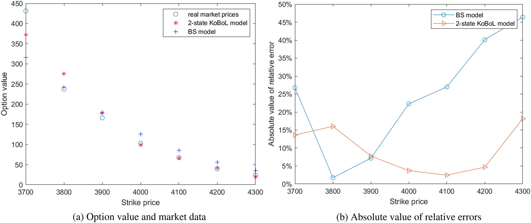
Comparison between two models.

From Figure 1(a), the option prices of the two-state KoBoL model are closer to the real market price. And from Figure 1(b), the absolute value of the relative error of the two-state KoBoL model is smaller than that of the BS model, although there are some sudden movements in the real-world market. It is clear that the two-state KoBoL model is better, and many fundamental empirical facts of financial markets, such as skewed and unexpected huge swings in stock prices, are explained by it.

In Table 4, the GMRES methods with two preconditioners and three different methods are compared with these parameters. It is clear that although the GMRES method using the Strang preconditioner P m (21) has improved a lot of iterations, the GMRES method using the proposed preconditioner P (10) with the Sherman-Morrison formula is still the best in terms of both iterations and CPU time in this case.

Table 4

Iteration numbers and CPU time of three methods for Example 3

N	M	IM-nP		IM-P		IM-b-P
		Ite	CPU	Ite	CPU	Ite	CPU
2 8	2 4	183.2	0.30 s	6.0	0.03 s	5.0	0.02 s
2 9	2 5	32.7	0.20 s	6.0	0.05 s	5.0	0.03 s
2 10	2 6	15.2	0.28 s	5.0	0.13 s	5.0	0.10 s
2 11	2 7	11.2	0.74 s	5.8	0.44 s	5.0	0.43 s

5 Conclusion

In this study, the regime-switching European option pricing based on the fractional diffusion model is studied. In order to reduce the calculation cost of solving the model, a second-order scheme of the implicit finite difference method is used, the analysis of related stability and convergence is given, and a special structure coefficient matrix is provided. The proposed preconditioner of the generalized minimal residual method solves the linear system M x = b , which is accelerated by FFT. And then the Sherman-Morrison formula and ILU factorization are used to improve the calculation efficiency. Besides, the rationality of this preconditioner is also ensured by the theoretical analysis and finally proves the effectiveness of the proposed second-order scheme with the block preconditioner through numerical examples including an empirical example.

In addition, since the application of the Sherman-Morrison formula is limited by the number of states J ¯ , the GMRES method using the proposed preconditioner P (10) with the Sherman-Morrison formula is chosen when J ¯ is 2 and the GMRES method with the preconditioner P (10) using ILU factorization is chosen when J ¯ is large.

Acknowledgement

The authors would like to express their sincere thanks to the referees for their valuable suggestions that led to an improved version of this manuscript.

Funding information: This work was supported in part by research grants of University of Macau (File Nos. MYRG2020-00208-FST and MYRG2022-00262-FST), Guangdong Basic and Applied Basic Foundation (Grant No. 2020A1515110991), the National Natural Science Foundation of China (Grant No. 12101137), and the Science and Technology Development Fund, Macau SAR under Funding Scheme for Postdoctoral Researchers of Higher Education Institutions 2021 (File No. 0032/APD/2021).
Author contributions: All authors have accepted responsibility for the entire content of this manuscript and approved its submission.
Conflict of interest: The authors state no conflict of interest.
Data availability statement: All data generated or analysed during this study are included in this published article.

References

[1] F. Black and M. Scholes, The pricing of options and corporate liabilities, J. Pol. Econ. 81 (1973), no. 3, 637–654, DOI: https://doi.org/10.1086/260062. 10.1086/260062Search in Google Scholar

[2] R. C. Merton, Theory of rational option pricing, Bell J. Econ. Manage. Sci. 4 (1973), 141–183, DOI: https://doi.org/10.2307/3003143. 10.2307/3003143Search in Google Scholar

[3] S. G. Kou, A jump-diffusion model for option pricing, Manage. Sci. 48 (2002), no. 8, 955–1101, DOI: https://doi.org/10.1287/mnsc.48.8.1086.166. 10.1287/mnsc.48.8.1086.166Search in Google Scholar

[4] P. Carr and L. Wu, The finite moment log stable process and option pricing, J. Finance 58 (2003), no. 2, 753–777, DOI: https://doi.org/10.1111/1540-6261.00544. 10.1111/1540-6261.00544Search in Google Scholar

[5] P. Carr, H. Geman, D. B. Madan, and M. Yor, The fine structure of asset returns: An empirical investigation, J. Bus. 75 (2002), no. 2, 305–332, DOI: https://doi.org/10.1086/338705. 10.1086/338705Search in Google Scholar

[6] S. I. Boyarchenko and S. Z. Levendorskiĭ, Non-Gaussian Merton-Black-Scholes Theory, Statistical Science & Applied Probability, Vol. 9, World Scientific, Singapore, 2002. 10.1142/4955Search in Google Scholar

[7] S. L. Heston, A closed-form solution for options with stochastic volatility with applications to bond and currency options, Rev. Financ. Stud. 6 (1993), no. 2, 327–343, DOI: https://doi.org/10.1093/rfs/6.2.327. 10.1093/rfs/6.2.327Search in Google Scholar

[8] R. J. Elliott and C. J. U. Osakwe, Option pricing for pure jump processes with Markov switching compensators, Finance Stoch. 10 (2006), no. 2, 250–275, DOI: https://doi.org/10.1007/s00780-006-0004-6. 10.1007/s00780-006-0004-6Search in Google Scholar

[9] P. Asiimwe, C. W. Mahera, and O. Menoukeu-Pamen, On the price of risk under a regime switching CGMY process, Asia-Pac. Financ. Mark. 23 (2016), 305–335, DOI: https://doi.org/10.1007/s10690-016-9219-5. 10.1007/s10690-016-9219-5Search in Google Scholar

[10] D. Hainaut and O. Le Courtois, An intensity model for credit risk with switching Lévy processes, Quant. Finance 14 (2014), no. 8, 1453–1465, DOI: https://doi.org/10.1080/14697688.2012.756583. 10.1080/14697688.2012.756583Search in Google Scholar

[11] G. Deelstra and M. Simon, Multivariate European option pricing in a Markov-modulated Lévy framework, J. Comput. Appl. Math. 317 (2017), 171–187, DOI: https://doi.org/10.1016/j.cam.2016.11.040. 10.1016/j.cam.2016.11.040Search in Google Scholar

[12] S. Lei, W. Wang, X. Chen, and D. Ding, A fast preconditioned penalty method for American options pricing under regime-switching tempered fractional diffusion models, J. Sci. Comput. 75 (2018), no. 3, 1633–1655, DOI: https://doi.org/10.1007/s10915-017-0602-9. 10.1007/s10915-017-0602-9Search in Google Scholar

[13] X. Li, P. Lin, X. C. Tai, and J. Zhou, Pricing two-asset options under exponential Lévy model using a finite element method, arXiv:1511.04950v1, 2015, https://doi.org/10.48550/arXiv.1511.04950.Search in Google Scholar

[14] X. He and S. Lin, A fractional Black-Scholes model with stochastic volatility and European option pricing, Expert Syst. Appl. 178 (2021), 114983, DOI: https://doi.org/10.1016/j.eswa.2021.114983. 10.1016/j.eswa.2021.114983Search in Google Scholar

[15] X. Chen, D. Ding, S. Lei, and W. Wang, An implicit-explicit preconditioned direct method for pricing options under regime-switching tempered fractional partial differential models, Numer. Algorithms 87 (2021), no. 3, 939–965, DOI: https://doi.org/10.1007/s11075-020-00994-7. 10.1007/s11075-020-00994-7Search in Google Scholar

[16] S. Lin and X. J. He, A regime switching fractional Black-Scholes model and European option pricing, Commun. Nonlinear Sci. Numer. Simul. 85 (2020), 105222, DOI: https://doi.org/10.1016/j.cnsns.2020.105222. 10.1016/j.cnsns.2020.105222Search in Google Scholar

[17] A. Cartea and D. del Castillo-Negrete, Fractional diffusion models of option prices in markets with jumps, Phys. A 374 (2007), no. 2, 749–763, DOI: https://doi.org/10.1016/j.physa.2006.08.071. 10.1016/j.physa.2006.08.071Search in Google Scholar

[18] Z. Zhou, J. Ma, and X. Gao, Convergence of iterative Laplace transform methods for a system of fractional PDEs and PIDEs arising in option pricing, East Asian J. Appl. Math. 8 (2018), no. 4, 782–808, DOI: https://doi.org/10.4208/eajam.130218.290618. 10.4208/eajam.130218.290618Search in Google Scholar

[19] W. Chen, X. Xu, and S. P. Zhu, Analytically pricing European-style options under the modified Black-Scholes equation with a spatial-fractional derivative, Quart. Appl. Math. 72 (2014), no. 3, 597–611, DOI: https://doi.org/10.1090/S0033-569X-2014-01373-2. 10.1090/S0033-569X-2014-01373-2Search in Google Scholar

[20] W. Chen and S. Wang, A penalty method for a fractional order parabolic variational inequality governing American put option valuation, Comput. Math. Appl. 67 (2014), no. 1, 77–90, DOI: https://doi.org/10.1016/j.camwa.2013.10.007. 10.1016/j.camwa.2013.10.007Search in Google Scholar

[21] X. Guo, Y. Li, and H. Wang, Tempered fractional diffusion equations for pricing multi-asset options under CGMYe process, Comput. Math. Appl. 76 (2018), no. 6, 1500–1514, DOI: https://doi.org/10.1016/j.camwa.2018.07.002. 10.1016/j.camwa.2018.07.002Search in Google Scholar

[22] M. Chen and W. Deng, High order algorithms for the fractional substantial diffusion equation with truncated Lévy flights, SIAM J. Sci. Comput. 37 (2015), no. 2, A890–A917, DOI: https://doi.org/10.1137/14097207X. 10.1137/14097207XSearch in Google Scholar

[23] R. H. Chan and X. Jin, An introduction to iterative Toeplitz solvers, Fundamentals of Algorithms, Vol. 5, SIAM, Philadelphia, 2007. 10.1137/1.9780898718850Search in Google Scholar

[24] S. L. Lei, D. Fan, and X. Chen, Fast solution algorithms for exponentially tempered fractional diffusion equations, Numer. Methods Partial Differential Equations 34 (2018), no. 4, 1301–1323, DOI: https://doi.org/10.1002/num.22259. 10.1002/num.22259Search in Google Scholar

[25] M. S. Bartlett, An inverse matrix adjustment arising in discriminant analysis, Ann. Math. Statist. 22 (1951), 107–111, DOI: https://doi.org/10.1214/aoms/1177729698. 10.1214/aoms/1177729698Search in Google Scholar

Received: 2023-09-15

Revised: 2023-12-07

Accepted: 2023-12-07

Published Online: 2023-12-31

This work is licensed under the Creative Commons Attribution 4.0 International License.

Articles in the same Issue

https://doi.org/10.1515/math-2023-0169

Keywords for this article

fully implicit finite difference method; preconditioner; regime-switching European option pricing; tempered fractional partial differential equation

Creative Commons

BY 4.0