An analysis on the stability of a state dependent delay differential equation

Sertaç Erman; Ali Demir

doi:10.1515/math-2016-0038

Enjoy 40% off

academic books on De Gruyter Brill *

Article Open Access

An analysis on the stability of a state dependent delay differential equation

Sertaç Erman and Ali Demir

Published/Copyright: June 23, 2016

Published by

Become an author with De Gruyter Brill

Submit Manuscript Author Information Explore this Subject

$Open Mathematics$

From the journal Open Mathematics Volume 14 Issue 1

Abstract

In this paper, we present an analysis for the stability of a differential equation with state-dependent delay. We establish existence and uniqueness of solutions of differential equation with delay term τ(u(t))=a+bu(t)c+bu(t). Moreover, we put the some restrictions for the positivity of delay term τ(u(t)) Based on the boundedness of delay term, we obtain stability criterion in terms of the parameters of the equation.

Keywords: Asymptotic stability; state depended delay; delay differential equation

MSC 2010: 34K20; 34K05

1 Introduction

Delay differential equations (DDE) have been used in many fields for a long time. However, state-dependent delay differential equations (SDDE) are used to make more realistic modelling in the systems whose delay varies according to the internal effects of the system. For example, the length of time to maturity is taken as constant delay in a simple population dynamics model, see in [1]. In [2], it was observed that the length of time to maturity of Antarctic whales and seals alter according to the state of the population and it was analyzed by using a mathematical model with SDDE in [3]. In addition, mathematical models with SDDE appear in many fields such as physics, control theory, neural network, medicine, biology etc., see Section 2 in [4] as a review.

Researchers have investigated SDDE for the last 50 years. Driver [5, 6] and Driver and Norris [7] developed a fundamental theory and proved local existence and uniqueness theorem for SDDE having Lipschitz continuous initial functions. Winston [8] showed that SDDE has a unique solution under some conditions in addition to continuos initial function. There are some of the earliest studies on SDDE in [9–11]. Moreover, many researches on stability, bifurcations and existence of solutions of SDDE have been done so far, for example, [3, 4, 12–31]. Especially, [32] can be seen as a detailed review on DDE and SDDE and related studies.

In this paper, we consider the following type of SDDE

u′(t)=−A0u(t)−A1u(t−τ(u(t)))(1)

where A₀, A₁ ∈ ℝ and τ(u(t)) > 0 for all t ∈ ℝ⁺. To analyze stability of solution of equation (1), we use the following characteristic equation

g(λ)=λ+A0+A1e−λh=0(2)

where h is an independent real valued parameter which is in the range of τ(u(t)). By this way, we analyze the stability of equation (1) by using the stability analysis of certain linear delay differential equations with constant delay which has the characteristic equation (2).

In the general case, the characteristic roots λ_j, j = 1, 2, ···, of equation (1) are obtained by solving the characteristic equation (2) where λ_j is a complex number. If the characteristic roots have negative real parts, i.e., Re(λ_j) < 0 for all j = 1, 2, ··· then the solution of (1) is asymptotically stable and if at least one of the characteristic roots have positive real parts, i.e., Re(λ_j) > 0 for some j = 1, 2, ··· then the solution of (1) is unstable.

We attempt to determine the stability and instability regions of the system in parameter space (A₀, A₁) by using D-partition method. The method is originated from paper [33]. It is well explained in [34–38] and analysis are conducted. Let’s consider the characteristic equation g(λ, A₀, A₁) in two parameters for equation (1). D-partition method is based on fact that the roots of the characteristic equation are continuos functions of the parameters A₀ and A₁. When varying the parameters, λ_j change continuously in complex plane and at the point where the stability changes, one λ_j crosses the imaginary axis. In this method parameter space is divided into regions with the hypersurfaces. These hypersurfaces are called the D-curves. The points of the D-curves correspond to pure imaginary roots or zero root of the characteristic equation. Moreover, in each region in the parameter space determined by the D-curves, the characteristic equation has the same number of roots with positive real part. Thus, finding the number of roots with positive real parts for specific point is enough to find the number of roots with positive real parts the region including this specific point.

In order to obtain D-curves, pure imaginary number λ = iω is substituted in characteristic equation g(λ, A₀, A₁). Equating to zero the real and imaginary parts, we have

U(ω,A0,A1)=Re(g(iω,A0,A1))=0(3)

V(ω,A0,A1)=Im(g(iω,A0,A1))=0(4)

Hence, by making use of (3) and (4), parametric equations can be written as

A0=A0(ω) A1=A1(ω)

where ω is a parameter and ranges from –∞ to ∞. These curves and singular solutions of equations (3) and (4) constitute D-curves.

We use Rekasius transform

e−iωh=1−iωT1+iωT for h=2ω(arctan(ωT)+pπ)(5)

where h, T ∈ ℝ and for p ∈ ℤ in addition to D-partition method. In 1980, Rekasius [39] proposed the transformation (5) for DDEs. Later, Thowsen [40] did exact calculations by taking the square of right hand side of (5) since the transformation (5) transform a circle to a semi-circle which leads some mistakes. However, Hertz et al. [41] did exact calculations by considering two singular cases:

(i) e^–iωh = –1 for T = ±∞

(ii) e^–iωh = 1 for T = 0

Olgaç and Sipahi [42, 43] studied a method using Rekasius transform for DDE with constant delay.

We establish the existence and uniqueness of solutions of equation (1) with delay term τ(u(t))=a+bu(t)c+bu(t) where a, b, c, d ∈ ℝ such that a and c are nonzero and at least one of b or d is nonzero, under certain condition in Section 2. In Section 3, by using D-partition method and transformation (5), conditions for the stability of equation (1) are presented.

2 Existence and uniqueness of solution

In this section, we consider the following type of SDDE

u′(t)=−A0u(t)−A1u(t−τ(u(t)))τ(u(t))=a+bu(t)c+du(t)>0,∀t∈ℝ+(6)

where A₀, A₁ ∈ ℝ⁺, a, b, c, d ∈ ℝ such that a and c are nonzero and at least one of b or d is nonzero.

Let P(u(t)) = a + bu(i) and Q(u(t)) = c + du(t). σ=−ab,μ=−cd be the roots of P(x) and Q(x) respectively. If one of the following conditions

i) u(t) > or u(t) < μ when sign(b) sign(d) = 1 and μ < σ,

ii) u(t) > μ or u(t) < when sign(b) sign(d) = 1 and σ < μ,

iii) μ < u(t) < σ when sign(b) sign(d) = –1 and μ < σ,

iv) σ < u(t) < μ when sign(b) sign(d) = –1 and σ < μ, is satisfied then τ(u(t)) ≥ 0.

In order to guarantee the positivity of delay term τ(u(t)), we need to put some restrictions on the range of parameter values under consideration.

Theorem 2.1

Let A₀, A₁ ∈ ℝ⁺and τ(u(t)) be delay function of equation(6). The delay differential equation

u′(t)=−A0u(t)−A1u(t−τ˜(u(t)))τ˜(u(t))=max{0,τ(u(t))}≥0for all t∈ℝ+(7)

has a unique solution u(t) ∈ C¹([0, ∞) → (L₀, M₀)) if Lipschitz history function u₀(t): [–τ, 0] → (L₀, M₀) exists such that

(L0,M0)={(σ,−σA1A0);μ<σ<0(−σA1A0);0<σ<μ(σ,μ);σ<0<μ,−σA1A0<μ(μ,σ);μ<0<σ,μ<−σA1A0(8)

andτ=maxu(t)∈(L0,M0)(τ˜(u(t))).

Proof. For the proof, the following four cases are considered.

Case 1: Let’s prove that u(t) ∈ (L₀, M₀) for all t > 0 when μ < σ < 0. Suppose not, then there exists t₀ > 0 such that u(t) ∈ (L₀, M₀) for all t < t₀ but u(t₀) = L₀ or u(t₀) = M₀. First assume that u(t₀) = L₀ which implies u′(t₀) ≤ 0. On the other hand

u(t0−τ˜(u(t0)))=u(t0)=σ

and

u′(t0)=−A0u(t0)−A1u(t0−τ˜(u(t0)))=−σ(A1+A0)>0

which is a contradiction. In a similar way, if u(t₀) = M₀, then u′(t₀) ≥ 0. On the other hand

u′(t0)=−A0u(t0)−A1u(t0−τ˜(u(t0)))<A0σA1A0−A1σ=0

which is a contradiction.

Case 2: Let’s prove that u(t) ∈ (L₀, M₀) for all t > 0 when 0 < σ < μ. Suppose not, then there exists t₀ > 0 such that u(t) ∈ (L₀, M₀) for all t < t₀ but u(t₀) = L₀ or u(t₀) = M₀. First assume that u(t₀) = L₀ which implies u′(t₀) ≤ 0. On the other hand

u′(t0)=−A0u(t0)−A1u(t0−τ˜(u(t0)))>A0σA1A0−A1σ=0

which is a contradiction. In a similar way, if u(t₀) = M₀, then u′(t₀) ≥ 0. On the other hand

u′(t0)=−A0u(t0)−A1u(t0−τ˜(u(t0)))=−σ(A1+A0)<0

which is a contradiction.

Case 3: Let’s prove that u(t) ∈ (L₀, M₀) for all t > 0 when σ<0<μ,−σA1A0<μ. Suppose not, then there exists t₀ > 0 such that u(t) ∈ (L₀, M₀ – ɛ) for all t < t₀ but u(t₀) = L₀ or u(t₀) = M₀ – ɛ for ɛ >0. First assume that u(t₀) = L₀ which implies u′(t₀) ≤ 0. On the other hand

u(t0−τ˜(u(t0)))=u(t0)=σ

and

u′(t0)=−A0u(t0)−A1u(t0−τ˜(u(t0)))=−σ(A1+A0)>0

which is a contradiction. In a similar way, if u(t₀) = M₀ – ɛ for ɛ > 0, then u′(t₀) ≥ 0. On the other hand

u′(t0)=−A0u(t0)−A1u(t0−τ˜(u(t0)))<−A0(μ−ε)−A1σ<A0σA1A0+A0ε−A1σ=A0ε

which is a contradiction since u(t₀) and A₀ɛ tend to μ and 0 respectively when ɛ tends to 0.

Case 4: Let’s prove that u(t) ∈ (L₀, M₀) for all t > 0 when μ < 0 < σ, μ<−σA1A0. Suppose not, then there exists t₀ > 0 such that u(t) ∈ (L₀ + ɛ, M₀) for all t < t₀ but u(t₀) = L₀ + ɛ for ɛ > 0 or u(t₀) = M₀. First assume that u(t₀) = L₀ + ɛ for ɛ > 0 which implies u′(t₀) ≤ 0. On the other hand

u′(t0)=−A0u(t0)−A1u(t0−τ˜(u(t0)))>−A0(μ−ε)−A1σ>A0σA1A0+A0ε−A1σ=−A0ε

which is a contradiction since u(t₀) and A₀ɛ tend to μ and 0 respectively when ɛ tends to 0. In a similar way, if u(t₀) = M₀, then u′(t₀) ≥ 0. On the other hand

u′(t0)=−A0u(t0)−A1u(t0−τ˜(u(t0)))=−σ(A1+A0)<0

which is a contradiction. As a result, there is no such t₀ ∈ ℝ⁺ and (8) holds.

Since

f(t,u,ν)=−A0u(t)−A1ν(t),α(t,u))=t−a+bu(t)c+du(t)

are Lipschitz with respect to each of their argument, local existence and uniqueness of the solution u(t) follows from Driver [5]. □

Theorem 2.2

Let A₀, A₁ ∈ ℝ⁺such thatA02−A12≥0and τ(u(t)) be delay function of equation(6). The delay differential equation(7)has a unique solution u(t) ∈ C¹[(0, ∞) → (L₀, M₀)), if Lipschitz history function u₀(t) : [–τ, 0] → (L₀, M₀) exists such that

(L0,M0)={(−μA0A1);0<μ≤σ or σ<0<μ,−σA1A0≥μ(μ,−μA0A1);σ≤μ<0 or μ<0<σ,μ≥−σA1A0(9)

andτ=maxu(t)∈(L0,M0)(τ˜(u(t))).

Proof. For the proof, following two cases are considered.

Case 1: Let’s prove that u(t) ∈ (L₀, M₀) for all t > 0 when 0 < μ ≤ σ or σ < 0 < μ, −σA1A0≥μ. Suppose not, then there exists t₀ > 0 such that u(t) ∈ (L₀, M₀ – ɛ) for all t < t₀ but u(t₀) = L₀ or u(t₀) = M₀ – ɛ for ɛ > 0. First assume that u(t₀) = L₀ which implies u′(t₀) ≤ 0. On the other hand

u′(t0)=−A0u(t0)−A1u(t0−τ˜(u(t0)))>μ(A02−A12)A1>0

which is a contradiction. In a similar way, if u(t₀) = M₀ – ɛ for ɛ > 0, then u′(t₀) ≥ 0. On the other hand

u′(t0)=−A0u(t0)−A1u(t0−τ˜(u(t0)))<−A0μ+A0ε+A1μA0A1=A0ε

which is a contradiction since u(t₀) and A₀ɛ tend to μ and 0 respectively when ɛ tends to 0.

Case 2: Let’s prove that u(t) ∈ (L₀, M₀) for all t > 0 when σ ≤ μ < 0 or μ < 0 < μ,μ≥−σA1A0. Suppose not, then there exists t₀ > 0 such that u(t) ∈ (L₀ + ɛ, M₀) for all t < t₀ but u(t₀) = L₀ + ɛ for ɛ > 0 or u(t₀) = M₀. First assume that u(t₀) = L₀ + ɛ for ɛ > 0 which implies u′(t₀) ≤ 0. On the other hand

u′(t0)=−A0u(t0)−A1u(t0−τ˜(u(t0)))>−A0μ−A0ε+A1μA0A1=−A0ε

which is a contradiction since u(t₀) and A₀ɛ tend to μ and 0 respectively when ɛ tends to 0. In a similar way, if u(t₀) = M₀, then u′(t₀) ≥ 0. On the other hand

u′(t0)=−A0u(t0)−A1u(t0−τ˜(u(t0)))<μ(A02A12A1<0

which is a contradiction. As a result, there is no such t₀ ∈ ℝ⁺ and (9) holds.

Since

f(t,u,ν)=−A0u(t)−A1ν(t),α(t,u))=t−a+bu(t)c+du(t)

are Lipschitz with respect to each of their argument, local existence and uniqueness of the solution u(t) follows from Driver [5]. □

If the delay functions τ(u(t)) and τ˜(u(t)) are equal to each other for u(t) ∈ (L₀, M₀), Theorems 2.1 and 2.2 also hold for the equation (6).

Corollary 2.3

Let’s be(L0,M0)=(σ−σA1A0)for μ < σ ≤ 0 or(L0,M0)=(−σA1A0,σ)for 0 < σ < μ and sign(b) sign(d) = 1. Equation(6)has a unique solution u(t) ∈ C¹.([0, ∞) → (L₀, M₀)) where τ is defined in Theorem 2.1 with Lipschitz history function u₀(t) : [–τ, 0] → (L₀, M₀).

Corollary 2.4

Let’s be(L0,M0)=(−μA0A1,μ)for 0 < μ ≤ σ or(L0,M0)=(μ−μA0A1)for σ ≤ μ < 0 sign(b) sign(d) = 1. Equation(6)has a unique solution u(t) ∈ C¹.([0, ∞) → (L₀, M₀)) where τ is defined in Theorem 2.2 with Lipschitz history function u₀(t) : [–τ, 0] → (L₀, M₀) and under the conditionA02−A12≥0.

Corollary 2.5

Let’s be (L₀, M₀) = (σ, μ) forσ<0<μ<−σA1A0<μor (L₀, M₀) = (μ, σ) for μ < 0 < σ, μ<−σA1A0and sign(b) sign(d) = –1. Equation(6)has a unique solution u(t) ∈ C¹.([0, ∞) → (L₀, M₀)) where τ is defined in Theorem 2.1 with Lipschitz history function u₀(t) : [–τ, 0] → (L₀, M₀).

Corollary 2.6

Let’s be(L0,M0)=(−μA0A1,μ)forσ<0<μ<−σA1A0≥μor(L0,M0)=(μ,−μA0A1)forμ<0<σ,μ≥−σA1A0and sign(b) sign(d) = –1. Equation(6)has a unique solution u(t) ∈ C¹ ([0, ∞) → (L₀, M₀)) where τ is defined in Theorem 2.2 with Lipschitz history function u₀(t) : [–τ, 0] → (L₀, M₀) and under the conditionA02−A12≥0.

In the case of d = 0 the Theorem 2.2 does not hold and the last two intervals in (8) in Theorem 2.1 do not longer exist. Moreover, if d = 0, c = 1, a > 0 and b > 0 then by Theorem 2.1, the solution exists in the interval (σ−σA1A0) which was previously found in [22].

These results allow us to do stability analysis of solution of (1) by using the range of τ(u(t)) which is obtained by Theorems 2.1 and 2.2.

Furthermore, if the delay function τ(u(t)) has a complicated form, then [1/1] Padé approximation for τ(u(t)) can be obtained and the stability analysis can be done by using rough range of τ(u(t)) which is obtained by the range of the solution u(t) approximately by the help of Theorems 2.1 and 2.2. The same can be done, if the delay function τ(u(t)) is not known exactly but some of its suitable values are obtained by some experiments or a heuristic method.

3 Stability analysis

In this section, we firstly consider the stability of equation (1) with the delay function τ(u(t)) which has an upper bound for all t ∈ ℝ⁺, i.e., there exist at least one M₁ ∈ ℝ such that 0 < τ(u(t)) < M₁ for all t ∈ ℝ⁺.

In this case, the value of delay of equation (1) varies in interval (0, M₁) while t is varying. The independent parameter h of the characteristic equation (2) takes values in the interval (0, M₁). As a part of the D-partition method, we have

C*:A0+A1=0 for λ=0(10)

this straight line is a line forming the boundary of the D-partition and is denoted by C_*. Substituting λ = iω and equating to zero the real and imaginary parts in characteristic equation (2), we find the following equations

A0+A1cos(ωh)=0(11)

ω+A1sin(ωh)=0.(12)

Solving the above equations for A₀ and A₁, the following parametric curve equations are obtained

A0(ω,h)=−ωcos(ωh)sin(ωh)(13)

A1(ω,h)=ωsin(ωh).(14)

Since A₀(ω, h/ and A₁(ω, h) are even with respect to ω, it is sufficient to take ω ∈ (0, ∞). Equations (13)-(14) define a family of curves since h is not a constant. Holding h fixed, these define A₀(ω, h) and A₁(ω, h) as function of ω, providing a parametric representation of a curve. Different values of h give different curves in the family. Since equations (13)-(14) have singularity for ωh = kπ, we introduce intervals Jk=(kπh,(k+1)πh) and denote by C_k(h) the curve in the parameter space (A₀, A₁) for ω ∈ J_k.

C₀(h) contains the limit point for ω → 0

(limω→0A0(ω,h),limω→0A1(ω,h))=(−1h,1h).(14)

In addition, the following limits can be obtained for k ∈ ℕ – {0}

limω→((2k−1)πh)−A0(ω,h)=limω→((2k−1)πh)−A1(ω,h)=limω→((2kπ)h)−A0(ω,h)=limω→((2kπ)h)+A1(ω,h)=+∞limω→((2k−1)πh)+A0(ω,h)=limω→((2k−1)πh)+A1(ω,h)=limω→((2kπ)h)+A0(ω,h)=limω→((2kπ)h)+A1(ω,h)=−∞

Lemma 3.1

The curves C₀(h) intersect C_*exactly once at(−1h,1h)for each positive number h. Moreover, C_k(h) do not intersect C_*for k ∈ ℕ – {0}:

Proof. Intersection of C₀(h) and C_* is obvious from (15). For the second part of Lemma 3.1, suppose that if C_k(h) and C_* has intersection points there exist ω ∈ J_k for equations (13)-(14) which satisfies equation (10). By using equations (13)-(14) in equation (10) we have

ωcos(ωh)sin(ωh)=ωsin(ωh).

There is no solution ω ∈ J_k for k ∈ ℕ – {0} which is a contradiction. □

Lemma 3.2

The curves C_k(h₀) do not intersect each other for h₀ ∈ ℝ⁺.

Proof. Suppose that there exist an intersection point. It means that, there exist ω₁ ≠ ω₂ ∈ ℝ⁺ such that A₀(ω₁, h₀) = A₀(ω₂, h₀) and A₁(ω₁, h₀) = A₁(ω₂, h₀). These equalities imply that

ω1sin(ω1h0)=ω2sin(ω2h0)ω1cos(ω1h0)sin(ω1h0)=ω2cos(ω2h0)sin(ω2h0)(16)

from equation (13) and (14). For n ∈ ℕ, ω₁h₀ ≠ ω₂h₀ + 2nπ is obtained from the left equality in (16) because of ω₁ ≠ ω₂: In addition, left and right equalities in (16) lead to cos(ω₁h₀) = cos(ω₂h₀) which is a contradiction. □

Lemma 3.3

The curve C_k(h₀) intersects the line A₀ = 0 exactly once for h₀ ∈ ℝ⁺. Moreover, the intersection point (0, P_k) satisfies the following inequalities

Pk<Pk+2 for =2n, n∈ℕPk+2<Pk for k=2n+1, n∈ℕ.

Proof. When ω ∈ J_k, the equation A₀(ω, h₀) = 0 implies ω=π+2kπ2h0.Hence,

Pk={π+2kπ2h0 for k=2n, n∈ℕ−π+2kπ2h0 for k=2n+1, n∈ℕ.

is obtained by substituting ω=π+2kπ2h0. This completes the proof. □

Theorem 3.4

The solution of equation

u′(t)=−A0u(t)−A1u(t−h), for h∈ℝ+(17)

is asymptotically stable, i.e., all the roots of equation

λ+A0+A1e−λh=0(18)

have negative real parts, if and only if

(a) −1h<A0

(b) −A0<A1<ωsin(ωh)where ω is the root ofA0=−ωcos(ωh)sin(ωh)such that ωh ∈ (0, π)

Proof. When A₀ > 0 and A₁ = 0, the solution of equation is clearly asymptotically stable. The stability region which includes half line A₀ > 0 and A₁ = 0, lies above C_* and below C₀(h) because of Lemmaa 3.1, 3.2 and 3.3. The conditions (a)–(b) are algebraic representation of this region in parameter space (A₀, A₁).

To find the number of roots with positive real parts in each region in the parameter space determined by the D-curves, we use the following the ideas from [38]. Writing λ = μ + iω with μ, ω ∈ ℝ in characteristic equation g(λ, A₀, A₁), we find two real equations

G1(μ,ω,A0,A1):=Re(g(μ,ω,A0,A1))=0(19)

G2(μ,ω,A0,A1):=Im(g(μ,ω,A0,A1))=0(20)

for the real and imaginary parts of λ. Direction of movement of an element is determined by the following proposition, using Jacobian matrix J defined by

J=[∂G1∂A0∂G1∂A1∂G2∂A0∂G2∂A1]μ=0

Proposition 3.5

The pure imaginary roots enter the right half-plane for parameters sets in the (A₀, A₁) parameter region to the left of the D-curves, when we follow this curve in the direction of increasing ω, whenever det(J) < 0 and to the right when det(J) > 0 [38].

Since the determinant of Jacobian matrix of equation (18) satisfies the following inequalities

det(J)<0 ω∈J2kdet(J)>0 ω∈J2k+1,

the pure imaginary roots move into the right half-plane when moving away in the parameter space to the left of C_2k(h) and to the right of C_2k+1(h), with "left" and "right" as determined w.r.t. a counter clock-wise tracking of C_2k(h) and a clock-wise tracking of C_2k+1(h) respectively.

In Fig. 1 these results are illustrated for h = 1. The curves (13) and (14) and the straight line (10) form the D-partition are shown and the number of roots in the right half plane is indicated for each region.

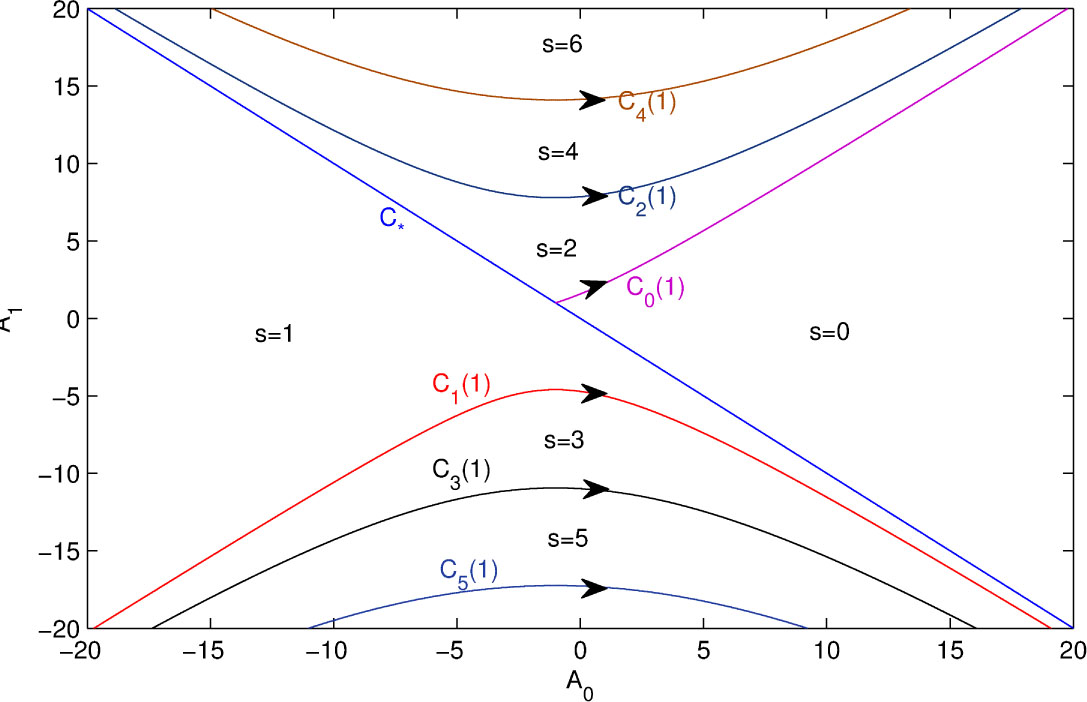
$Fig. 1 The member of the D-curves family Ck(h) in the parameter space (A0, A1) for h = 1. The arrows along the curves refer to the direction of increasing ω. The numbers s in the different regions bordered by the curves indicate the number of roots in the right half plane.$

Fig. 1

The member of the D-curves family C_k(h) in the parameter space (A₀, A₁) for h = 1. The arrows along the curves refer to the direction of increasing ω. The numbers s in the different regions bordered by the curves indicate the number of roots in the right half plane.

Until Theorem 3.4, parameter is taken as a real constant. Now we determine how stability region varies when h is varying.

Lemma 3.6

The members of family of curves C_k(h) do not intersect each other for k ∈ ℕ. Proof. Suppose that there exists an intersection point for h₁ < h₂. It means that, there exist ω₁h₁, ω₂h₂ ∈ (kπ, (k + 1)π) such that

ω1cos(ω1h1)sin(ω1h1)=ω2cos(ω2h2)sin(ω2h2)(21)

ω1sin(ω1h1)=ω2sin(ω2h2).(22)

Cos(ω₁h₁) = cos(ω₂h₂) is obtained by using (21) and (22) which implies that ω₁h₁ = ω₂h₂ because of ω₁h₁, ω₂h₂ ∈ (kπ, (k + 1)π). Therefore we have ω₁ ≠ ω₂ from the assumption h₁ < h₂ which contradicts (22).

Lemma 3.7

If h₁ < h₂, C₀(h₂) lies below C₀(h₁) in parameter space (A₀, A₁).

Proof. Taking the derivative of (13) and (14) with respect to h, we obtain

∂A0∂h=ω2sin2(ωh)∂A1∂h=−ω2cos(ωh)sin2(ωh).

It implies that, A₀(ω, h) is a monotone increasing function and A₁(ω, h) is a monotone decreasing function for ωh∈(0,π2). For each ωh value, functions A₀(ω, h) and A₁(ω, h) represent coordinates of points on C₀(h). Therefore, if h₁ < h₂, the point (A₀(ω, h₂), A₁(ω, h₂)) lies below the point (A₀(ω, h₁), A₁(ω, h₁)) for ωh₁, ωh2∈(0,π2). Suppose that a part of C₀(h₂) lies above C₀(h₁) for ωh₁, ωh2∈[π2,π), then there exists at least one intersection point of C₀(h₂) and C₀(h₁), which contradicts Lemma 3.6. □

The curves C₀(h) are shown for h = 0:25; 0:75, 1, 1:3 in Fig. 2.

$Fig. 2 The members of the D-curves family C0(h) in the parameter space (A0, A1) for h = 0:25, 0:5, 0:75, 1 and 1:3$

Fig. 2

The members of the D-curves family C₀(h) in the parameter space (A₀, A₁) for h = 0:25, 0:5, 0:75, 1 and 1:3

Proposition 3.8

Let’s define the set S_h as follows

Sh={(A0,A1)|A0,A1∈ℝ and satisfy the conditions (a) and (b) for h∈ℝ+.}

If h₁ < h₂then S_h₁ ⊂ S_h₂.

Proof. It is clear from Lemma 3.7

Theorem 3.9

The solution of equation(1)with delay term τ(u(t)) > 0 which satisfies the condition 0 < τ(u(t)) < M₁for all t ∈ ℝ⁺is asymptotically stable if and only if the following conditions are satisfied:

(ã) −1M1<A0

(b˜)−A0<A1<ωsin(ωM1)where ω is the root ofA0=−ωcos(ωM1)sin(ωM1)such that ωM₁ ∈ (0, π)

Proof. It is obvious form Theorem 2.1 and Proposition 3.8 that if the conditions. (ã) and (b˜) are satisfied, all roots of characteristic equation of equation (1) have negative real parts. □

Definition 3.10

A delay value of DDE is called critical delay if DDE has pure imaginary or zero eigenvalues at this delay value.

Critical delays of an equation are the values at which the qualitative behavior of the system changes. Between any two successive critical values, the behavior of the solution does not change.

Now, by using transformation (5) we rewrite the critical delay values of equation (17) in terms of parameter.

Proposition 3.11

λ = iω is a root of equation(18)for some h if and only if λ = iω is also a root of

Tλ2+(1+A0T−A1T)λ+A0+A1=0(23)

for some T ≥ 0

Proof. Let λ = iω be a root of equation (18). By using transformation (5) in equation (18), we obtain

iω+A0+A11−iωT1+iωT=0.

Multiplying this equation by 1 + iωT and arranging properly, we get

T(iω)2+(1+A0T−A1T)iω+A0+A1=0

which implies that λ = iω is a root of equation (23) for h=2ω(arctan(ωT)+pπ). Moreover, the singular cases of Rekasius transform (5) are satisfied for equation (16) and equation (21).

As a result, T=1A1−A0,ω=±A12−A02 and critical delays

hp=2A12−A02(arctan(A12−A02A1−A0+pπ)),p∈ ℤ

are obtained under the condition |A₀| < A₁. Let h_n denote least h_p value which is greater than 0. Therefore, the solution of equation (17) is stable for h ∈ (0, h_n) when 0 < A₀ < A₁. Hence we can state the following result about stability of the solution for the equation (1).

Theorem 3.12

The solution of the equation(1)with delay τ(u(t)) > 0 such that 0 < τ(u(t)) < M₁for all t ∈ ℝ⁺is asymptotically stable under the conditions |A₀| < A₁and M₁ < h_n.

Now, we give a stability criterion which is independent from delay for equation (1) by using D-partition method.

Theorem 3.13

If |A₁| < A₀, then the solution of equation (1) is asymptotically stable.

Proof. It is obvious from (11) that, |A₁(ω)| ≥ |A₀(ω)| for all ω ∈ J_k. Therefore, all of the D-curves is in this region, i.e., there is no D-curve in the region described by |A₁| < |A₀|. Moreover, the half line A₀ > 0 and A₁ = 0 on which the solution equation (1) is asymptotically stable, is in the region described by |A₁| < A₀.

4 Conclusion

In this study, we have analyzed the stability of a differential equation with state-dependent delay under some conditions which guarantee existence and uniqueness of solutions. For the positivity of delay term τ(u(t))=a+bu(t)c+du(t), we put the some restrictions on the range of parameters values under consideration.

We consider two cases according to the boundedness of delay term. In the first case, the delay term is supposed to be bounded and we have two theorems, namely Theorems 3.9 and 3.12, related to stability of the solution. It is shown that upper bound of the delay term affects the stability region of differential equation with state-dependent delay: smaller upper bound means greater stability region. Moreover, by using the Rekasius transform, which is an analytic transformation, we get equation (23) which is equivalent to the characteristic equation of a differential equation with state-dependent delay. In the second case, the delay term is supposed to be unbounded and we have a theorem, namely Theorem 3.13. It is shown that we can find a stability region for the solution, even though the delay term is unbounded, since there is a stability region which is independent from delay term.

In the future we would like to investigate the stability of differential equation with different state-dependent delay. This would allow for a better understanding of differential equation with state-dependent delay.

References

[1] Murray J.D., Mathematical biology I. An introduction, 3rd ed, Springer-Verlag, Berlin Heidelberg, 2002.Search in Google Scholar

[2] Gambell R., Birds and mammals-Antarctic whales in Antarctica, W. N. Bonner and D. W. H.Walton, eds., Pergamon Press, New York, 1985, 223-241.10.1016/B978-0-08-028881-9.50022-4Search in Google Scholar

[3] Aiello W.G., Freedman H.I., Wu J., Analysis of a model representing stage-structured population growth with statedependent time delay, SIAM J Appl Math, 1992, 52, 855–869.10.1137/0152048Search in Google Scholar

[4] Hartung F., Krisztin T., Walther H.O., Wu J. Functional differential equations with state-dependent delays: theory and applications, A. Canada, P. Drabek, A. Fonda, Eds., Handbook of Differential Equations: Ordinary Differential Equations, vol. III, Elsevier/North-Holland, Amsterdam, 2006, 435–545.10.1016/S1874-5725(06)80009-XSearch in Google Scholar

[5] Driver R.D., Existence theory for a delay-differential system, Contrib Differential Equations, 1963, 1, 317–336.Search in Google Scholar

[6] Driver R.D., A two-body problem of classical electrodynamics: the one-dimensional case, Ann Physics, 1963, 21, 122–142.10.1016/0003-4916(63)90227-6Search in Google Scholar

[7] Driver R.D., Norris M.J., Note on uniqueness for a one-dimensional two-body problem of classical electrodynamics, Ann Physics, 1967, 42, 347–351.10.1016/0003-4916(67)90076-0Search in Google Scholar

[8] Winston E., Uniqueness of solutions of state dependent delay differential equations, J Math Anal Appl, 1974, 47, 620–625.10.1016/0022-247X(74)90013-4Search in Google Scholar

[9] Cooke K.L., Asymptotic theory for the delay-differential equation u_(t)=-au(t -r(u(t))), J Math Anal Appl, 1967, 19, 160–173.10.1016/0022-247X(67)90029-7Search in Google Scholar

[10] Nussbaum R.D., Periodic solutions of some nonlinear autonomous functional differential equations, Ann Mat Pura Appl, 1974, 101, 263–306.10.1007/BF02417109Search in Google Scholar

[11] Alt W., Some periodicity criteria for functional differential equations, Manuscripta Math, 1978, 23, 295–318.10.1007/BF01171755Search in Google Scholar

[12] Mallet-Paret J., Nussbaum R.D., Paraskevopoulos P. Periodic solutions for functional differential equations with multiple state-dependent time lags, Topol. Methods Nonlinear Anal, 1994, 3, 101–16210.12775/TMNA.1994.006Search in Google Scholar

[13] Krisztin T., An unstable manifold near a hyperbolic equilibrium for a class of differential equations with state-dependent delay, Discrete Contin Dyn Syst, 2003, 9, 993–102810.3934/dcds.2003.9.993Search in Google Scholar

[14] Sieber J., Finding periodic orbits in state-dependent delay differential equations as roots of algebraic equations, Discrete Contin Dyn Syst Ser A, 2012, 32, 2607–265110.3934/dcds.2012.32.2607Search in Google Scholar

[15] Hu Q., Wu J., Global Hopf bifurcation for differential equations with state-dependent delay, J Differ Equ, 2010, 248, 2081–284010.1016/j.jde.2010.03.020Search in Google Scholar

[16] Hartung F., Differentiability of solutions with respect to the initial data in differential equations with state-dependent delay, J Dyn Differ Equ, 2011, 23, 843–88410.1007/s10884-011-9218-1Search in Google Scholar

[17] Arino O., Hadeler K.P., Hbid M.L. Existence of periodic solutions for delay differential equations with state-dependent delay, J Differ Equ, 1998, 144, 263–30110.1006/jdeq.1997.3378Search in Google Scholar

[18] Kuang Y., Smith H.L. Slowly oscillating periodic solutions of autonomous state-dependent delay differential equations, Nonlinear Anal Theory Methods Appl., 1992, 19, 855–87210.1016/0362-546X(92)90055-JSearch in Google Scholar

[19] Mallet-Paret J., Nussbaum R.D., Boundary layer phenomena for differential-delay equations with state-dependent time-lags: I, Arch Ration Mech Anal, 1992, 120, 99–14610.1007/BF00418497Search in Google Scholar

[20] Mallet-Paret J., Nussbaum R.D., Boundary layer phenomena for differential-delay equations with state-dependent time-lags: II, J Reine Angew Math, 1996, 477, 129–19710.1007/BF00418497Search in Google Scholar

[21] Mallet-Paret J., Nussbaum R.D., Boundary layer phenomena for differential-delay equations with state-dependent time-lags: III, J Differ Equ, 2003, 189, 640–69210.1016/S0022-0396(02)00088-8Search in Google Scholar

[22] Mallet-Paret J., Nussbaum R.D. Superstability and rigorous asymptotics in singularly perturbed state-dependent delay-differential equations, J Differ Equ, 2011, 250, 4037–4084.10.1016/j.jde.2010.10.024Search in Google Scholar

[23] Magal P., Arino O. Existence of periodic solutions for a state-dependent delay differential equation, J Differ Equ, 2000, 165, 61–95.10.1006/jdeq.1999.3759Search in Google Scholar

[24] Krisztin T., Arino O., The 2-dimensional attractor of a differential equation with state-dependent delay, J Dyn Differ Equ, 2001, 13, 453–522.10.1023/A:1016635223074Search in Google Scholar

[25] Kennedy B., Multiple periodic solutions of an equation with state-dependent delay, J Dyn Differ Equ, 2011, 26, 1–31.10.1007/s10884-011-9205-6Search in Google Scholar

[26] Stumpf E., On a differential equation with state-dependent delay: a global center-unstable manifold connecting an equilibrium and a periodic orbit, J Dyn Differ Equ, 2012, 24, 197–24810.1007/s10884-012-9245-6Search in Google Scholar

[27] Walther H.-O., A periodic solution of a differential equation with state-dependent delay, J Differ Equ, 2008, 244, 1910–1945.10.1016/j.jde.2008.02.001Search in Google Scholar

[28] Cooke K., Huang W., On the problem of linearization for state-dependent delay differential equations, Proc Am Math Soc, 1996, 124, 1417–1426.10.1090/S0002-9939-96-03437-5Search in Google Scholar

[29] Chueshov I., Rezounenko A., Dynamics of second order in time evolution equations with state-dependent delay, Nonlinear Analysis, 2015, 126–149.10.1016/j.na.2015.04.013Search in Google Scholar

[30] Rezounenko A., On time transformations for differential equations with state-dependent delay, Cent. Eur. J. Math., 2014, 12(2), 298-307.10.2478/s11533-013-0341-6Search in Google Scholar

[31] Otrocol D., Ilea V., Ulam stability for a delay differential equation, Cent. Eur. J. Math., 2013, 11(7), 1296-1303.10.2478/s11533-013-0233-9Search in Google Scholar

[32] Walther H.-O., Topics in Delay Differential Equation, Jahresber Dtsch Math-Ver, 2014, 116, 87–114.10.1365/s13291-014-0086-6Search in Google Scholar

[33] Neimark J.I., D-subdivision and spaces of quasi-polynomials (in Russian), Prikl Mat Mekh, 1949, 13, 349–380.Search in Google Scholar

[34] Elsgolts L.E., Norkin S.B. Introduction to the Theory and Application of Differential Equations with Deviating Arguments, Academic Press, London, 1973.Search in Google Scholar

[35] Insperger T., Stépán G., Semi-Discretization Stability and Engineering Applications for Time-Delay Systems, Springer, Newyork, 2011.10.1007/978-1-4614-0335-7Search in Google Scholar

[36] Kolmanovskii V.B., Nosov V.R., Stability of Functional Differential Equations, Academic Press, London, 1986.Search in Google Scholar

[37] Krall A.M. Stability Techniques for Continuous Linear Systems, Gordon and Breach, Newyork, 1967.Search in Google Scholar

[38] Diekmann O., Gils S.A. van, Lunel S.M.V., Walther H.-O. Delay Equations, Functional, Complex and Nonlinear Analysis, Springer, New York, 1995.10.1007/978-1-4612-4206-2Search in Google Scholar

[39] Rekasius Z., A stability test for systems with delays, Proc of joint Autom Contr Conf San Francisco, 1980.Search in Google Scholar

[40] Thowsen A., An analytic stability test for class of time-delay system, IEEE Trans. Autom. Control, 1981, 26(3), 735–736.10.1109/TAC.1981.1102694Search in Google Scholar

[41] Hertz J.D., Jury E., Zeheb E., Simplified analytic stability test for systems with commensurate time delays, IEE Proc Part D, 1984, 131, 52–56.10.1049/ip-d.1984.0008Search in Google Scholar

[42] Olgaç N., Sipahi R., An exact method for the stability analysis of time-delayed linear time-invariant (LTI) systems, IEEE Trans. Autom. Control, (2002), 47(5), 793–797.10.1109/TAC.2002.1000275Search in Google Scholar

[43] Sipahi R., Olgaç N., A unique methodology for the stability robustness of multiple time delay systems, Syst Control Lett, 2006, 55(10), 819–825.10.1016/j.sysconle.2006.03.010Search in Google Scholar

Received: 2016-3-21

Accepted: 2016-5-30

Published Online: 2016-6-23

Published in Print: 2016-1-1

This work is licensed under the Creative Commons Attribution-NonCommercial-NoDerivatives 3.0 License.