What is ‘advanced statistical modelling’?: commentary on “Replication and methodological robustness in quantitative typology” by Becker and Guzmán Naranjo

A long-standing challenge in quantitative typological studies has been to correctly account for two fundamental features of the world’s languages: their similarities with other languages due to genealogical relationships and shared inheritance, and their similarities with other languages due to language contact and borrowing. Past approaches have often included geographical units like continents, known areas of contact (Bickel and Nichols 2006; Nichols et al. 2013) or language families as random effects in mixed-effects models. Bootstrapping methods across these geographic areas or families have also been considered. B&GN’s (Becker and Guzmán Naranjo 2025) advocacy for replication in quantitative typology leads them to emphasize a more refined approach: a phylogenetic Bayesian regression with a “geographic” Gaussian process. The former accounts for the tree-like nature of linguistic genealogies, while the latter captures the spatiality of language contact. This approach is convincingly and pedagogically declined across several case studies, and sets a solid benchmark for future studies.

The authors describe their models as “advanced statistical techniques” for bias control, and we wish to emphasize three complementary aspects of this expression. Each suggests recommendations to possibly follow in future publications.

First, the authors’ approach to replication does not consist in replacing one model with another, but rather with a series of complementary models whose comparison offers insights into the situation. This contrastive approach highlights the weight of different predictors in a comprehensive manner, which is especially useful when these predictors overlap in their effect. When it comes to linguistics, languages in contact are often also genealogically close, and it is hard to disentangle effects of inheritance from effects of borrowing. Given a set of key predictors of a linguistic distribution, considering (a) no connection between languages, (b) language contact only, (c) phylogeny only or (d) both contact and phylogeny could be done more systematically to characterize what underlies the observed situation. Showing in particular the predictions of different models, as in Figure 5 of the paper, strengthens understanding through more explicit representations. It is also worth paying close attention, when the data includes them, to areas where languages in contact are not all closely related genealogically, such as the Balkan Sprachbund, the Caucasus, South-East Asia etc. (Hartmann and Jäger 2023).

As the authors put it, there is no simple best way to analyse a given dataset. In addition to the previous complementary sets of predictors, we should encourage, when it makes sense, considering a few alternative modelling options and assessing their convergence.

For instance, for the Gaussian process, the authors relied on a specific kernel – also known as covariance function (Görtler et al. 2019) – to capture how two languages are related given the distance between them (computed on the basis of their geographic coordinates). Their choice, the so-called “exponentiated quadratic kernel”, assumes a specific shape for the decay in the influence of languages on each other as their distance increases. This might not be, however, the best option to capture the effect of geographic distance, and other shapes might be considered. Figure 1 illustrates three possible options (among many others). The “exponential kernel” (in red) assumes a stronger decay than the squared exponential kernel (in blue) for shorter distances, while the “rational quadratic kernel” (in green) suggests a slower decay overall. One could compare these different kernels and find which one best captures the data under study.

Figure 1:

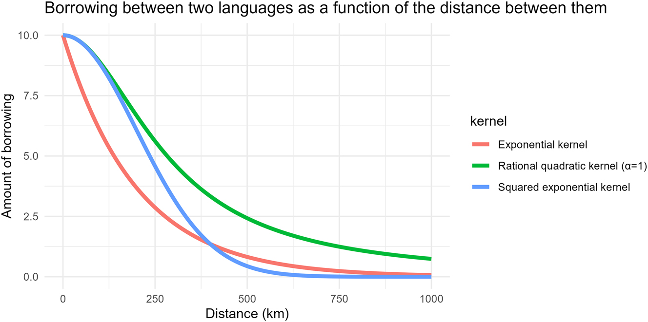
Different possible kernels for a Gaussian process accounting for the influence of geographic distance between two languages (the numerical scale for the amount of borrowing is defined for the sake of illustration and does not relate to any existing data).

If several conceptually valid models all point in the same direction – for instance, they all suggest that a predictor has a strong and significant effect – this lends additional confidence to such a result. It shows indeed that a specific modelling choice, like the kernel of a Gaussian process, does not determine the outcomes of the model. The point is not here to try several models in search of one that returns what one expects to find, as this would increase the chances of false positives. Rather, one may consider several models as integral to their approach.

Second, the authors rely on different “types” of models, namely a nominal/categorical regression, a 0–1 inflated beta regression model, and a multivariate beta regression model with correlated phylogenetic effects.^[1] Considering such models requires a solid understanding of statistics, extending beyond well-known statistical tests (chi², t-test, ANOVA etc.) and the widely used multiple linear regression and logistic regression. The point here is that the model must match how the predicted variable is distributed given the predicting variables under consideration – what is known as its conditional distribution. Failure to do so means that the output of the model cannot be trusted. As an example, applying a linear regression model to predict the decay factor in Seržant’s (2021) study would not raise any kind of error when running the code, as there is no mathematical impossibility. However, an assumption of the linear regression is that the conditional mean of the predicted value is an affine function of the predictors, which is often not the case for frequency values. When that is not the case, the residuals, i.e., the differences between the actual values of the predicted variable and the predictions of the model, won’t appear to be normally distributed as they should. A quantile–quantile plot, or Q–Q plot, of the residuals is often used to visually assess the situation: the dots should be aligned if the distribution is normal.

To illustrate this point, we contrasted B&GN’s m_cline model in the replication of Seržant’s study with a linear regression model with the same predictor (latitude). Figure 2 shows the Q-Q plots of the residuals for the two models. The non-alignment of the dots for the linear regression suggests that this model is not very appropriate for the data, more specifically for the small values close to 0. By contrast, the 0–1 inflated beta regression offers well-aligned dots.

Figure 2:

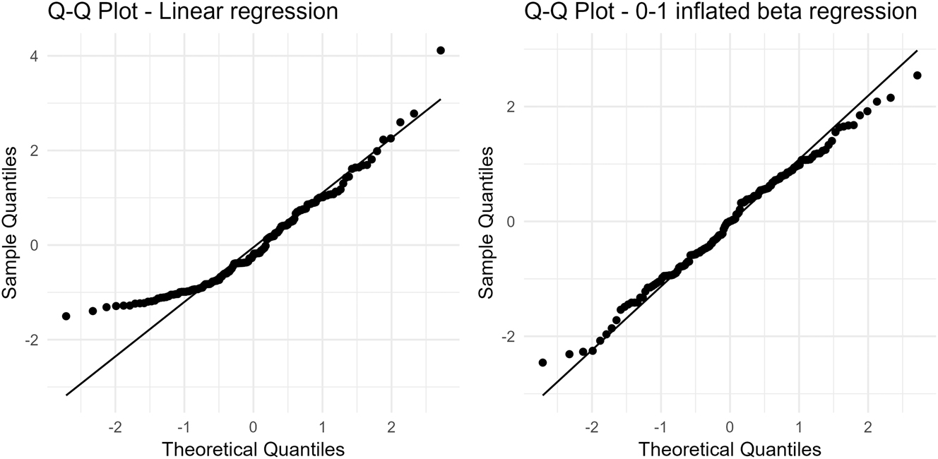
Q–Q plots for two regression models predicting Seržant’s decay factor with latitude. The models were computed with the gamlss2 package in R (https://github.com/gamlss-dev/gamlss2). The residuals are quantile residuals, which are expected to follow a standard normal distribution when the model is correctly specified.

It is not common at all to see authors report that they have verified that the assumptions of their model(s) were met. This should become a standard requirement, as one among different sanity checks.

Once again, there is no simple best way to analyse a given dataset, but some modelling options make more sense than others and should thus be preferred. In the case of the multivariate beta regression model with correlated phylogenetic effects, a simpler approach would be to consider two independent beta regressions and forget that the two predicted variables are both under the influence of the same phylogenetic relationships. This choice would likely not violate the assumptions of the two beta regressions. But if one tries to better account for how the values of the two predicted variables are distributed – their overall variance – the authors’ choice of model is more meaningful. Finding more sensible options is about being more knowledgeable about the wide range of options offered by statistics. Paying attention to other fields where geography and phylogeny matter – ecology in particular – can prove fruitful here.^[2] For instance, different linguistic families appear to have their own rate of evolution (Nevalainen et al. 2020), but the phylogenetic component in B&GN’s models assumes that the rate of linguistic evolution is always the same along the different branches of the language tree. It is possible to relax this constraint/assumption (Davies et al. 2019), and therefore build a model that better matches the history of languages. Similarly, a simple “geographic” Gaussian process assumes that the relationship between linguistic influence and geographic distance – the shape of the decay illustrated in Figure 1 – is the same wherever on the planet. It is reasonable to think, nevertheless, that this is not the whole story (Huisman et al. 2019). For instance, different physical environments likely differ in how distance impacts language contact: deserts or rugged mountainous terrains likely make interactions at greater distances more challenging and less frequent. Nettle (1996, 1998) also suggested that climatic variability and ecological risk play a key role in the size of sociolinguistic networks. Once again, recent models (Du et al. 2020) offer the possibility to relax the assumption of stationarity in the geographic space, i.e., the assumption that the impact of distance does not depend on where the languages are located. This helps to be more faithful to the complex reality of language contact.

Third, statistical models express a phenomenon through the values for their parameters. In a simple linear regression model with one continuous predictor, which can be written as y = α + β x + ɛ – ɛ representing the error term –, only two values, those of the coefficient β and of the intercept α, need to be estimated. One needs enough observations in a dataset to reliably estimate the parameters of the model. To put it differently, for a given number of observations, the more parameters, the less confidence one can have regarding the estimation of these parameters and the predictions of the model. In statistical terms, it can be said that the total number of degrees of freedom provided by the data can be decomposed into the degrees of freedom “consumed” by the model and its parameters, and the number of residual degrees of freedom (often simply called the number of degrees of freedom), which relates to the statistical power of the model.

When considering regression to model language diversity, the willingness to highlight the role of additional factors, to account for non-linear phenomena, and to control for language genealogy and/or language contact, always lead to more complex models in the sense of a larger number of parameters having to be estimated. Modelling toolkits like STAN and brms offer here a lot of flexibility and temptations. As the authors rightly point out, we need to embrace the uncertainty that comes with more informational models, as it reflects the complexity of the phenomenon under study. The limit is, however, when our quest for comprehensiveness cannot be matched by the amount of data. At some point, the number of parameters to estimate can be too high to highlight true effects with good confidence. The model is then under-powered and p-values above the 0.05 threshold or Bayesian credible intervals including 0 are more likely to erroneously suggest that there is no effect. In addition to that, effects that do appear to be significant are more likely to be false positives. Uncertainty is not here part of the reality of the situation under study, but an issue with the model itself. Coming back once more to the idea that there is no simple best way to analyse a given dataset, a better approach may be out of reach given the available data.

The point is to differentiate between what is not significant but could be significant given the statistical power of the model, and what is not significant and could not be anyway. This requires a prospective power analysis. Power analyses, which help in particular to determine the smallest sample size needed for a research study (more specifically, for a required significance level, statistical power, and effect size), have become standard practice in fields like medicine, and are timidly making their way into linguistics (Vasishth 2023). While there are clear guidelines and methods for simpler statistical models, things nevertheless quickly become challenging as one adds smooth terms, correlation structures and other statistical treats (Cole and Abitante 2025). Different approaches, in particular simulation studies (Kumle et al. 2021), are gradually developed, and one can hope and recommend that they are eventually considered in quantitative typological studies.

The recommendations formulated in the previous paragraphs may seem challenging and excessive, but they can help push further our understanding of the intricacies of linguistic diversity. They certainly necessitate solid statistical knowledge and strong pedagogical efforts, of the kind and quality of those deployed by B&GN in their contribution. They suggest more frequent collaborations between linguists, who know what phenomena and factors should be considered, and statisticians, who can offer advice on if and how one may meet these demands.

References

Becker, Laura & Matías Guzmán Naranjo. 2025. Replication and methodological robustness in quantitative typology. Linguistic Typology 29(3). 463–505. https://doi.org/10.1515/lingty-2023-0076.Search in Google Scholar
Bickel, Balthasar & Johanna Nichols. 2006. Oceania, the Pacific Rim, and the theory of linguistic areas. Annual Meeting of the Berkeley Linguistics Society 32(2). 3–15. https://doi.org/10.3765/bls.v32i2.3488.Search in Google Scholar
Cole, David & George Abitante. 2025. Tips for estimating power in complex statistical models. https://www.psychologicalscience.org/publications/observer/estimating-power-statistical-models.html (accessed 6 April 2025).Search in Google Scholar
Davies, T. Jonathan, James Regetz, Elizabeth M. Wolkovich & Brian J. McGill. 2019. Phylogenetically weighted regression: A method for modelling non-stationarity on evolutionary trees. Global Ecology and Biogeography 28(2). 275–285. https://doi.org/10.1111/geb.12841.Search in Google Scholar
Du, Zhenhong, Zhongyi Wang, Sensen Wu, Feng Zhang & Renyi Liu. 2020. Geographically neural network weighted regression for the accurate estimation of spatial non-stationarity. International Journal of Geographical Information Science 34(7). 1353–1377. https://doi.org/10.1080/13658816.2019.1707834.Search in Google Scholar
Görtler, Jochen, Rebecca Kehlbeck & Oliver Deussen. 2019. A visual exploration of Gaussian processes. Distill 4. https://doi.org/10.23915/distill.00017.Search in Google Scholar
Gray, Russell D. & Quentin D. Atkinson. 2003. Language-tree divergence times support the Anatolian theory of Indo-European origin. Nature 426. 435–439. https://doi.org/10.1029/2001GC000192.Search in Google Scholar
Hartmann, Frederik & Gerhard Jäger. 2023. Gaussian process models for geographic controls in phylogenetic trees. Open Research Europe 3(57). https://doi.org/10.12688/openreseurope.15490.1.Search in Google Scholar
Huisman, John L. A., Asifa Majid & Roeland Van Hout. 2019. The geographical configuration of a language area influences linguistic diversity. PLoS One 14(6). https://doi.org/10.1371/journal.pone.0217363.Search in Google Scholar
Kumle, Levi, Melissa Lê-Hoa Võ & Dejan Draschkow. 2021. Estimating power in (generalized) linear mixed models: An open introduction and tutorial in R. Behavior Research Methods 53(6). 2528–2543. https://doi.org/10.3758/s13428-021-01546-0.Search in Google Scholar
Nettle, Daniel. 1996. Language diversity in West Africa: An ecological approach. Journal of Anthropological Archaeology 15. 403–438. https://doi.org/10.1006/jaar.1996.0015.Search in Google Scholar
Nettle, Daniel. 1998. Explaining global patterns of language diversity. Journal of Anthropological Archaeology 17. 354–374. https://doi.org/10.1006/jaar.1998.0328.Search in Google Scholar
Nevalainen, Terttu, Tanja Säily & Turo Vartiainen. 2020. Comparative sociolinguistic perspectives on the rate of linguistic change. Journal of Historical Sociolinguistics 6(2). 20200010. https://doi.org/10.1515/jhsl-2019-6001.Search in Google Scholar
Nichols, Johanna, Alena Witzlack-Makarevich & Balthasar Bickel. 2013. The AUTOTYP genealogy and geography database: 2013 release. http://www.spw.uzh.ch/autotyp/.Search in Google Scholar
Seržant, Ilja. 2021. Slavic morphosyntax is primarily determined by its geographic location and contact configuration. Scando-Slavica 67(1). 65–90. https://doi.org/10.1080/00806765.2021.1901244.Search in Google Scholar
Vasishth, Shravan. 2023. Some right ways to analyze (psycho)linguistic data. Annual Review of Linguistics 9(1). 273–291. https://doi.org/10.1146/annurev-linguistics-031220-010345.Search in Google Scholar
© 2025 the author(s), published by De Gruyter, Berlin/Boston
This work is licensed under the Creative Commons Attribution 4.0 International License.
Articles in the same Issue
- Frontmatter
- Target Paper and Discussion
- Introduction
- Replication, robustness and the angst of false positives: a timely target article and its multifaceted comments
- Target Paper
- Replication and methodological robustness in quantitative typology
- Commentaries
- Embracing uncertainty, and the multifaceted soul of linguistic typology: commentary on “Replication and methodological robustness in quantitative typology” by Becker and Guzmán Naranjo
- Replicability all the way up: commentary on “Replication and methodological robustness in quantitative typology” by Becker and Guzmán Naranjo
- Some comments on robustness in comparative grammar research: commentary on “Replication and methodological robustness in quantitative typology” by Becker and Guzmán Naranjo
- Open research requires open mindedness: commentary on “Replication and methodological robustness in quantitative typology” by Becker and Guzmán Naranjo
- An experimentalist’s perspective on replicability in typology: commentary on “Replication and methodological robustness in quantitative typology” by Becker and Guzmán Naranjo
- Sampling matters: commentary on “Replication and methodological robustness in quantitative typology” by Becker and Guzmán Naranjo
- Weak theories and robustness: commentary on “Replication and methodological robustness in quantitative typology” by Becker and Guzmán Naranjo
- Commentary: Replication, robustness or methodological competition?
- Good enough for Galton, and much more: commentary on “Replication and methodological robustness in quantitative typology” by Becker and Guzmán Naranjo