Rao-Blackwellizing field goal percentage

3.1 Measuring shot factors

In order to estimate shot-make probabilities, we first measure three shot factors based on how each shot entered the basket – left-right accuracy, depth, and entry angle – following the procedure of Marty and Lucey (2017). We define left-right accuracy as the deviation of the ball from the centre of the hoop as the ball crosses the plane of the basket (Figure 1A). Shot depth is defined as the distance of the ball from a tangent line through the front of the hoop as the ball crosses the plane of the basket (Figure 1A), with the front of the hoop adjusted to be from the perspective of the shooter. We specify the adjusted front of the rim as depth 0, so a shot crossing the basket plane at the center of the hoop has a depth of 9 inches. Finally, the entry angle is defined as the angle between the plane of the hoop and a tangent line through the ball as it is entering the basket (Figure 1B). See Marty and Lucey (2017) for further detail regarding these measurements.

Figure 1:

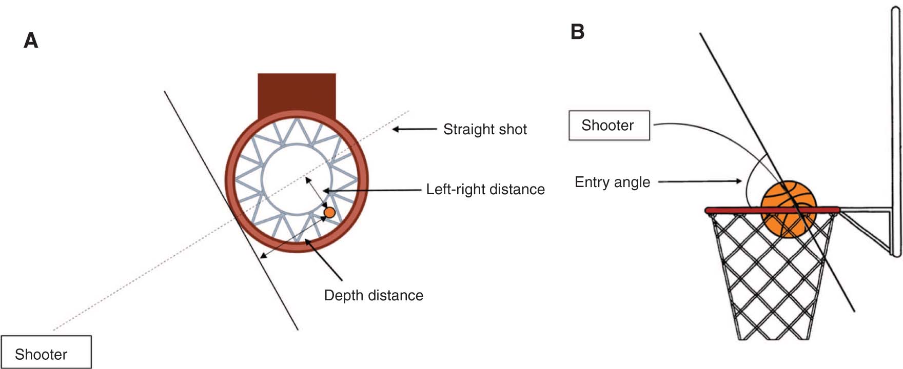
Shot factors at the plane of the hoop. (A) denotes the left-right and depth factors, (B) denotes the entry angle factor.

To obtain these shot factor estimates, we use shot trajectory information provided by the SportVu optical tracking data from STATS LLC. The data provides measurements of the X and Y coordinates for all 10 players and X, Y, and Z coordinates of the ball 25 times per second. Our dataset consists of 1212 games from the 2014–2015 NBA regular season and 1206 games from the 2015–2016 regular season. We first restrict our analysis to 3-point shots as these shots have the most trajectory information and we can assume all shooters are attempting to hit the centre of the basket (no shot attempts purposely off the backboard). In total our dataset consists of trajectory information for 47,631 3-point shots from the 2014–2015 season and 49,876 3-point shots from the 2015–2016 season.

Although the optical tracking data gives X, Y, and Z coordinates of the ball at the basket, the location data is noisy, especially in measuring the height of the ball. To obtain a better estimate of the position of the ball near the basket we model a quadratic best fit line through the trajectory data given by the tracking database. If Z_i is the height of shot i, and x_i and y_i are the X, Y coordinates of the shot in the tracking data, we use a quadratic polynomial to model the height, and estimate the coefficients by a least-squares regression:

We use the point where the model specifies the ball crosses 10 feet in height as the estimated X, Y location of the ball at the basket, and use this location to calculate the shot’s depth, left-right accuracy, and entry angle.

We compare the above model with a second model in which we try to leverage pre-existing knowledge of shot trajectories. We know each shot starts at the player’s location at the time of release (player location is less noisy than ball location in the tracking database) and ends around the basket. Therefore, we can improve estimation by biasing the start and end points of our modeled trajectories to incorporate this prior knowledge. To accomplish this we introduce a Bayesian regression model using pseudo-data to establish priors that reflect this knowledge. This is an informal empirical Bayes method where instead of using data to estimate the priors, we use prior knowledge of how the data should look. Given the quadratic model (1) for each shot, we can specify a Bayesian regression model with a conjugate Normal prior for β of the form ρ(β|σ2,z,X)∼N(u0,σ2Λ0−1). This results in a conjugate inverse gamma prior for σ² written as ρ(σ2|z,X)∼IG(a0,b0). We can then update our mean and precision parameters as:

where u_n is the posterior mean of β, and Λ_n is the posterior precision matrix for β. We update the parameters twice, once using pseudo-data reflecting our prior knowledge of where shots start and finish, and a second time using the shot trajectory data from the optical tracking data. We specify 4 pseudo-data points, 2 at the start of the shot set at the X, Y coordinates of the player when the shot is released and at a height of 7 feet, and 2 set at the centre of the hoop and at 10 feet in height. After two Bayesian learning updates we take the posterior mean of β, u₂, and use it as the estimate for the coefficients in the quadratic polynomial model (1).

We then use (1) to compute the 3 shot factors for each shot using both the ordinary linear regression (OLR) and Bayesian regression approaches. Comparing the two models, we find both predict shots to have a mean depth value of 11′′, a mean left-right value of 0′′, and a mean entry angle around 45°. As in Marty and Lucey (2017) we find shots entering the basket at 11′′ in depth, 2′′ deeper than the centre of the basket, and 0′′ in left-right accuracy are made with the highest percentage. However, we find shot depths are evenly distributed around 11′′, in contrast to the findings of Marty and Lucey (2017) who found that shooters have a mean shot depth value of 9′′, at the centre of the hoop. The variance in left-right distance and entry angle between the two models is similar, however the variance in shot depth is much larger in the OLR compared to the Bayesian regression model (Figure 2). Overall, variances in shot factors under the Bayesian model match the variances of the precise shot factor measurements of Marty and Lucey (2017) more closely than the OLR model. Furthermore, we will see later that when we model shot probabilities the Bayesian model produces a lower misclassification rate and log loss than the OLR model. Moving forward, we decide to use shot factors calculated via the Bayesian regression model.

Figure 2:

Estimated shot factor measurements under the ordinary and Bayesian regression models. Left/right and depth measurements are given as distance in feet in relation to the centre of the basket, where the depth of the centre of the basket is 0.75 feet. Entry angle measurements are given in radians to allow for the values to be on the same axis.

We next compare the precision of our estimated shot factors to those measured by the Noah Shooting System – a dedicated hardware install found in practice facilities that provides shooting information not available in live games. Marty and Lucey (2017) were able to use the Noah system to define a Guaranteed Make Zone (GMZ) of over 90% based on these shot factors. Their GMZ is marked by shots with an entry angle of 45°, a left-right accuracy between -2′′ and 2′′, and a depth between 7′′ and 14′′. Using our estimated shot factors, we found shots in this GMZ are made only 85.2% of the time. This suggests that despite the Bayesian model, our shot factor estimates are still less precise than those gathered by the Noah system.

3.2 Modeling shot-make probabilities

In this section we train a shot-make probability model using 3-point shots from the 2014–2015 season. To obtain shot-make probabilities for each shot, we use the estimated shot factors described previously as covariates in a logistic regression:

where S_i is an indicator function equal to 1 when a shot goes in and 0 went it misses, i indexes all 3-point shots from the 2014–2015 season (N = 47,631), σ(x)=exp(x)/(1+exp(x)), and D^_i, LR^_i, and Â_i are the estimated depth, left-right distance, and entry angle of shot i, respectively. We note that the Rao-Blackwell inequality indicates the framework detailed in Section 2 holds regardless of the choice of shot probability model, given the model provides reasonable estimates of shot probabilities.

Although our Bayesian regression model biases shot trajectories toward the basket, some trajectories are still quite variable. Modeled trajectories that are too far from the raw data are removed and instead assigned a probability of 1 or 0 for a make or miss, respectively. We use factors from the remaining shots to estimate shot-make probabilities with model (2). To assess how accurate the model is we perform a 10-fold cross-validation to obtain the mean misclassification rate, as well as calculate the log loss and Brier score. We repeat this procedure with shot factors estimated from the OLR model, and the results are shown in Table 1.

The covariates estimated via Bayesian regression resulted in misclassification rate 0.204. Therefore, our Bayesian model is able to predict makes/misses correctly about 80% of the time. This is a higher rate than many shot prediction models that use contextual covariates, like those presented in Cen et al. (2015) which utilize variables such as distance to basket and nearest defender to predict shot-makes with 65% accuracy. Similar to probabilities based on raw FG% (Marty and Lucey 2017), predicted shot-make probabilities are highest for shots at 11 inches depth, 0 inches of left-right deviation, and similar for shots with entry angles in the mid-40s. These can be seen in relation to the basket in Figure 3.

Figure 3:

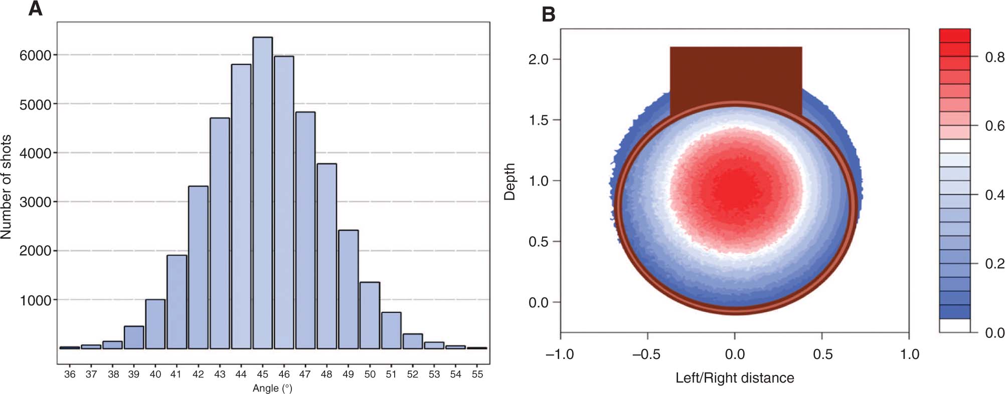
(A) shows the distribution of mean predicted shot-make probabilities over different shot entry angles. Included are all 3-point shots in the 2014–2015 season in which trajectory information is used to train our model (2). (B) shows the distribution of predicted shot-make probabilities over different values of shot depth and left-right accuracy in relation to the basket.

4.1 Predicting three-point field goal percentage

In this section we aim to create a new estimate for player FG% by aggregating estimated shot-make probabilities given by (2). Without loss of generality, we focus first on 3-point shots for clarity of presentation. We gather shot trajectories for 3-point shots taken from the first half of the 2015–2016 NBA season in the SportVu tracking database (N = 24,855), and predict the probability of each shot going in using model (2) trained by shots taken in the 2014–2015 season. The mean of these estimated shot-make probabilities is the RB-FG% estimate, θ^_RB, for each player’s FG%. We wish to see whether θ^_RB is better than raw FG%, θ^, at predicting a player’s future FG%, θ. We find that when predicting 3-point FG% in the second half of the 2015–2016 season, θ^_RB outperforms θ^ in terms of mean absolute error (Table 2). Interestingly, as seen similarly in Brown (2008), θ^ is quite a poor predictor of future shooting. It performs worse than simply using the league-wide grand mean as a predictor for every player (Table 2).

As mentioned in Section 2, due to the uncertainty in our shot factor estimates resulting from the noise in the optical tracking data, we do not know each shot’s true make probability. We can analyze how sensitive our estimator θ^_RB is to deviations in shot factor estimates by recalculating each shot’s depth, left-right accuracy, and entry angle based on sampling from the posterior distribution of the parameters in (1). We find that simulated estimates based on resampled shot factors perform nearly as well as those based on the mean parameter values from (1), and still vastly outperform raw FG% (Figure 4). Furthermore, we also find that the accuracy of our shot-make probability model (2) is important in determining the accuracy of θ^_RB. Removing the quadratic and interaction terms in (2) results in less accurate probability estimates, and we find this increases the mean absolute prediction error of θ^_RB from 0.0590 to 0.0608, respectively. However, this weakened estimator still outperforms raw FG%.

In addition to assessing prediction accuracy, we can also investigate whether the RB-FG% estimator produces more consistent player rankings than raw FG%. We calculate θ^ and θ^_RB for 3P% in the first and second half of the 2015–2016 season and rank all 260 players in our analysis according to each estimate. The θ^ and θ^_RB estimates produce Spearman’s rank coefficients of 0.216 and 0.245, respectively. We find, using the tests detailed in Fieller, Hartley, and Pearson (1957), that although RB-FG% produces a higher rank correlation than raw FG%, it is not significantly higher.

Figure 4:

The distribution of out-of-sample prediction errors for raw, Rao-Blackwellized (RB), simulated RB 3P%’s for 260 players from the 2015–2016 season. Errors are taken as the absolute difference between players’ (estimated) 3P% in the first half of the 2015–2016 season and their true 3P% in the second half of the season. The RB estimators are calculated by averaging shot-make probabilities given by (2). Simulated RB estimators are calculated in the same way as the RB case, except shot factors are measured by first resampling from the multivariate normal distribution on the parameters in (1) (rather than taking their mean as in the RB estimators). Players are separated by the number of 3-point shots attempted in the first half of the 2015–2016 season.

Rao-Blackwellizing the estimator for FG% does reduce variance and improve the prediction accuracy, but these estimators are based on low sample sizes for most players. Players in our dataset take between 3 and 402 three-point attempts in the first half of the 2015–2016 season, far fewer than the number needed for 3P% to stabilize (see Section 1). We are able to further reduce the variance of θ^_RB by introducing a empirical Bayesian shrinkage factor towards a Beta prior, B(α0,β0) (Casella 1985). We choose the hyperparameters of the Beta prior based on the posterior mean 3P% in the first half of the 2015–2016 season (0.35), and tune α₀ in terms of minimizing the mean absolute error of θ^_RB. We end up applying a prior distribution to each player’s first half 3-point shooting of the form B(3.5,6.5), in essence adding 10 league-average shots to θ^ and θ^_RB. Shrunk-RB estimates are calculated by the expected value of the updated Beta distribution as:

Table 2 shows that the shrunk-RB estimator is a better predictor than the shrunk-raw estimator, and this improvement is illustrated in Figure 5. Hence while Rao-Blackwellizing significantly improves prediction, leveraging knowledge about the distribution of 3P%’s can further improve the RB-FG% estimator (Efron and Morris 1977).

Figure 5:

Mean prediction error for the raw, Rao-Blackwellized, and shrunk-Rao-Blackwellized 3-point FG% estimators of 20 players in the first half of the 2015–2016 season. Errors are measured for predicting 3-point FG% in the second half of 2015–2016.

In addition to predicting future shooting, we can also use θ^_RB to estimate players’ 3P% with less data than when using θ^. The root-mean-square error (RMSE) of both estimators for inferring end-of-season 3P% is presented in Figure 6. RB-FG% has a lower RMSE than FG% when calculated using less than 30% of games, and the biggest improvements occur with low sample sizes. Some bias is introduced by RB-FG% as shot probabilities are modeled in (2) using the entire set of 3-point shots, while estimates are calculated seperately for each player. We only use a single set of priors to estimate shot factors in our Bayesian regression, but each player should have their own set of priors due to differences in height and shooting style. However, specifying individual priors and creating separate shot trajectory models for each player is difficult because most players take too few shots to obtain accurate parameter estimates. Additionally, the reduction in variance outweighs the small level of bias introduced by θ^_RB (Figure 6). Because we are comparing these estimators to raw FG% on the full sample, the raw estimator becomes better if we calculate RMSE using more than 40% of games. However, even full-season shooting numbers are highly variable and based on low sample sizes for most players. Thus RB-FG% is a better overall estimate on any size of data, but for small sample sizes it is a better estimate of end-of-season FG% than FG% itself.

Figure 6:

The RMSE of θ^ and θ^_RB estimating players’ true 3-point FG% for the 2014–2015 NBA season. These estimators are calculated using shots from a subset of games and compared to each player’s 3-point FG% at the end of the season. RMSE is calculated separately for each sub-box using 5%, 10%, 15%, 20%, 25%, and 30% of the games from the 2014–2015 season.

4.2 Predicting true shooting percentage

Although we’ve focused on three-point shots, we are able to Rao-Blackwellize any shooting statistic provided we have enough trajectory information to accurately estimate shot factors. We now expand our selection of shots and try to improve predictions of TS% using our shot factor and shot probability models. We repeat the procedure described in Section 3 to estimate shot factors for all two-point shots and free throws in the 2014–2015 season, and use these to create separate Rao-Blackwellized two-point FG% and free throw percentage (FT%) estimates. As before, shots that do not have enough location data or result in trajectory predictions very far from the raw data are not included in training or prediction datasets. In total, shot-make probabilities are estimated for 21,153 out of 24,832 free throws and 21,890 out of 73,925 two-point shots, with remaining probabilities assigned as 1 or 0 for a shot make and miss, respectively. The new RB estimators are again used to predict two-point FG%, FT% and TS% in the second half of the 2015–2016 season. As with 3P%, we find the shrunk Rao-Blackwellized estimator for TS% results in the lowest mean absolute error (Table 2).

Rao-Blackwellizing 2-point shots results in only a modest decrease in mean absolute error compared to the shrunk raw estimator. This may be because we are only able to estimate shot-make probabilities for a small fraction of two-point shots using the optical tracking database. Many 2-point shots are taken close to the basket or intended as bank-shots, resulting in insufficient or inaccurate trajectory information. These 2-point shots are not included in our prediction model and thus 2-point FG% is only partially Rao-Blackwellized. Interestingly, Rao-Blackwellizing FT% also resulted in only a minor improvement in prediction. This is not due to lack of trajectory information as most free throws are included in our shot-make model, but may be because free throws more closely follow a Bernoulli distribution than either 2-point or 3-point shots. Free throws are certainly more homogeous than other shot attempts as they are not affected by contextual factors like changing shot distance or defender pressure. There has been some research showing serial correlation between free throws (Arkes 2010). Though even when shown this effect is considerably smaller than the effects contextual factors have on field-goal shot-make probabilities. The closer that a player’s free throw attempts follow a Bernoulli distribution, the less potential there is to decrease the mean-squared error of the raw estimator of FT% through Rao-Blackwellization. If a player’s free throw attempts perfectly follow a Bernoulli distribution the number of makes and misses becomes a sufficient statistic for FT% and Rao-Blackwellizing would give no improvement in prediction accuracy.

4.3 Example of an improvement in inferring player FG%

We now present an example of when evaluating a player using θ^_RB instead of θ^ may change the interpretation of that player’s shooting and prediction of their future FG%. After signing with Miami Lebron James improved his 3-point shooting ability drastically, shooting 36.5% from three during the 2010–2011 to 2014–2015 seasons compared to just 32.9% in his first 7 seasons in Cleveland (Paine 2016). However, during the 2015–2016 season Lebron shot just 30.9% from three. Was there a real difference in his 3-point shooting ability during this season compared to the previous 5? If we attempt to answer this question using raw FG%, we can estimate a 90% confidence interval via a normal approximation of (0.264, 0.354). Thus with 90% confidence we can say there was a real difference between Lebron’s 3-point shooting during 2015–2016 compared to the previous 5 years. More traditional advanced metrics also fail to explain James’s dip in 3-point FG%. Compared to the 2014–2015 season (where James shot 35.4% from three), in 2015–2016 he shot from more favorable 3-point zones, shot fewer threes late in the shot clock, more of his threes came from assists, and fewer threes came against “tight” defensive pressure as classified by the SportVu tracking data (Paine 2016). All these indicators suggest that James’s 3-point shooting should have improved in 2015–2016, yet he shot his poorest percentage since his rookie year. Based on these statistics, one may have concluded that there was a real decrease in 3-point shooting skill during the 2015–2016 season, and we may have predicted that this poor shooting would continue in upcoming seasons. However, if we instead use RB-FG% as an estimator of 3P%, we estimate his 3-point percentage during 2015–2016 to be 34.7%, with a 90% confidence interval of (0.321, 0.374). Therefore, according to his RB-FG% Lebron did not have an appreciable decline in 3-point shooting ability, and we would predict that his FG% should revert back to somewhere around his average over the previous 5 years. As we’ve seen, this has indeed been the case as his 3P% returned to 36.3% and 36.7% during the 2016–2017 and 2017–2018 seasons, respectively.

References

Arkes, J. 2010. “Revisiting the Hot Hand Theory with Free Throw Data in a Multivariate Framework.” Journal of Quantitative Analysis in Sports 6(1): Retrieved 12 Jun. 2018, from doi:10.2202/1559-0410.1198.10.2202/1559-0410.1198Search in Google Scholar
Blackport, D. 2014. “How Long Does it Take for Three Point Shooting to Stabilize?” https://fansided.com/-2014/08/29/long-take-three-point-shooting-stabilize/. November 11th, 2017.Search in Google Scholar
Brown, L. D. 2008. “In-Season Prediction of Batting Averages: A Field Test of Empirical Bayes and Bayes Methodologies.” The Annals of Applied Statistics 2:113–152.10.1214/07-AOAS138Search in Google Scholar
Casella, G. 1985. “An Introduction to Empirical Bayes Data Analysis.” The American Statistician 39:83–87.10.1080/00031305.1985.10479400Search in Google Scholar
Chang, Y. H., R. Maheswaran, J. Su, S. Kwok, T. Levy, A. Wexler, and K. Squire. 2014. “Quantifying Shot Quality in the NBA.” Proceedings of the 2014 MIT Sloan Sports Analytics Conference.Search in Google Scholar
Cen, R., H. Chase, C. Pena-Lobel, and D. Silberwasser. 2015. “NBA Shot Prediction and Analysis.” https://hwchase17.github.io/sportvu/. November 11th, 2017.Search in Google Scholar
Efron, B., and C. Morris. 1977. “Stein’s paradox in statistics.” Scientific American 236:119–127.10.1038/scientificamerican0577-119Search in Google Scholar
Franks, A., A. D’Amour, D. Cervone, and L. Bornn. 2016. “Meta-Analytics: Tools for Understanding the Statistical Properties of Sports Metrics.” Journal of Quantitative Analysis in Sports 12:151–165.10.1515/jqas-2016-0098Search in Google Scholar
Fieller, E. C., H. O. Hartley, and E. S. Pearson. 1957. “Tests for rank correlation coefficients.” Biometrika 44:470–481.10.1093/biomet/44.3-4.470Search in Google Scholar
Kubatko, J., D. Oliver, K. Pelton, and D. T. Rosenbaum. 2007. “A Starting Point for Analyzing Basketball Statistics.” Journal of Quantitative Analysis in Sports 3(3): Retrieved 12 Jun. 2018, from doi:10.2202/1559-0410.1070.10.2202/1559-0410.1070Search in Google Scholar
Marty, R. 2018. “High-resolution Shot Capture Reveals Systematic Biases and an Improved Method for Shooter Evalutation.” Proceedings of the 2018 MIT Sloan Sports Analytics Conference.Search in Google Scholar
Marty, R. and S. Lucey. 2017. “A Data-Driven Method for Understanding and Increasing 3-Point Shooting Percentage.” Proceedings of the 2017 MIT Sloan Sports Analytics Conference.Search in Google Scholar
Paine, N. 2016. “LeBron’s 3-Point Shot Has Abandoned Him.” https://fivethirtyeight.com/features/lebrons-3-point-shot-has-abandoned-him/. January 3rd, 2018.Search in Google Scholar
Piette, J., A. Sathyanarayan, and K. Zhang. 2010. “Scoring and Shooting Abilities of NBA Players.” Journal of Quantitative Analysis in Sports 6(1): Retrieved 12 Jun. 2018, from doi:10.2202/1559-0410.1194.10.2202/1559-0410.1194Search in Google Scholar
Skellam, J. G. 1948. “A Probability Distribution Derived from the Binomial Distribution by Regarding the Probability of Success as Variable Between the Sets of Trials.” Journal of the Royal Statistical Society. Series B (Methodological) 10:257–261.10.1111/j.2517-6161.1948.tb00014.xSearch in Google Scholar
Young, S. 2016. “The NBA’s 3-point Revolution.https://bballbreakdown.com/2016/12/16/the-nba-3-point-revolution/. December 14th, 2017.Search in Google Scholar
©2019 Walter de Gruyter GmbH, Berlin/Boston
Articles in the same Issue