Local Entropy Production Rates in a Polymer Electrolyte Membrane Fuel Cell

Marc Siemer; Tobias Marquardt; Gerardo Valadez Huerta; Stephan Kabelac

doi:10.1515/jnet-2016-0025

Article Publicly Available

Local Entropy Production Rates in a Polymer Electrolyte Membrane Fuel Cell

Marc Siemer , Tobias Marquardt , Gerardo Valadez Huerta and Stephan Kabelac

Published/Copyright: July 23, 2016

Published by

Become an author with De Gruyter Brill

Submit Manuscript Author Information

From the journal Journal of Non-Equilibrium Thermodynamics Volume 42 Issue 1

Abstract

A modeling study on a polymer electrolyte membrane fuel cell by means of non-equilibrium thermodynamics is presented. The developed model considers a one-dimensional cell in steady-state operation. The temperature, concentration and electric potential profiles are calculated for every domain of the cell. While the gas diffusion and the catalyst layers are calculated with established classical modeling approaches, the transport processes in the membrane are calculated with the phenomenological equations as dictated by the non-equilibrium thermodynamics. This approach is especially instructive for the membrane as the coupled transport mechanisms are dominant. The needed phenomenological coefficients are approximated on the base of conventional transport coefficients. Knowing the fluxes and their intrinsic corresponding forces, the local entropy production rate is calculated. Accordingly, the different loss mechanisms can be detected and quantified, which is important for cell and stack optimization.

Keywords: non-equilibrium thermodynamics; fuel cell; entropy production; phenomenological equations

1 Introduction

Knowledge of the temperature, potential and concentration profiles within a polymer electrolyte membrane fuel cell (PEMFC) is essential for designing cooling strategies and for stack optimization. Transport processes for momentum, heat, charge and species are fundamental in order to determine these profiles across the fuel cell. Due to their physical nature, these transport processes are coupled. In the proton exchange membrane, this becomes especially clear, as e.g. the water transport due to the electroosmotic drag has an impact on the effective electrical resistance of the electrolyte and on the performance of the fuel cell [1, 2]. A reliable simulation model of a PEMFC should capture these coupling effects to accurately describe the heat, mass, momentum and charge transfer.

Conventional modeling approaches are well summarized in different reviews [3, 4]. One-dimensional fuel cell models similar to that proposed here are divided in different computational domains specified by their function. These domains are the gas channels, the gas diffusion layers (GDLs), the catalyst layers (CLs) and the electrolyte membrane. In the gas channel, the dominant transport process is convective mass and heat transfer. Due to the porosity of the GDL, the transport processes in this porous domain are often described by a diffusion term [5–7] (Fick- and Maxwell–Stefan-diffusion) combined with a convective term (Knudsen- and Darcy-diffusion). At the CL, the oxidation reaction

(1)H2→2H++2e−

At the anode, the reduction reaction

(2)12O2+2H++2e−→H2O

At the cathode, it takes place and their kinetics are described, e.g. with the Butler–Volmer equation [6, 8, 9]. Finally, the proton transport in the membrane is typically described by diffusion and electroosmosis [1, 5]. The transport and kinetic coefficients are often considered to be constant.

Transport of momentum, heat, charge and species is regularly described by relationships between forces and fluxes. Commonly it is assumed that only one force is responsible for a corresponding flux, e.g. a temperature gradient for transport of heat expressed by the law of Fourier. In most practical cases, this assumption is accurate enough. In some cases, however, coupled transport mechanisms have to be considered. This is the case for describing fuel cells and other electrochemical systems. Unfortunately, it is not always clear in advance, when this more accurate approach is needed. In reality, more than one forces contribute for a flux, as is well known from non-equilibrium thermodynamics. The fundamentals of this theory were established by Onsager [10] and Prigogine (see e.g. [11]). In this sense, a flux Ji is linearly correlated to the forces Xj as follows:

(3)Ji=∑j=1KLijXj

where the Lijs are the phenomenological coefficients and K is the number of the considered transport processes. The set of equations for all fluxes and forces are known as Onsager’s linear relationships or phenomenological equations.

Due to the irreversible nature of transport processes, the fluxes Ji and their intrinsic corresponding forces Xi are also correlated with the entropy production rate:

(4)σ=J1X1+J2X2+⋯

Knowing this entropy production is important to improve efficiencies, to predict hot spots and to build, e.g. better cooling strategies for a fuel cell or for a fuel cell stack.

A way of describing irreversible processes is to analyze the system with endoreversible thermodynamics, as proposed by Wagner et al. [12] and also implemented for a PEMFC model by the same authors [13]. In this sense, the system should be divided in reversible operating subsystems, which interact irreversibly with each other.

In this contribution, the PEMFC model is in part similar to the model of Wöhr et al. [14], but it is set up and analyzed by means of non-equilibrium thermodynamics. An approach to the entropy production similar to that proposed by Kjelstrup et al. [15] is used for our purpose.

2 Theory

The processes that occur in the different domains of the PEMFC induce heat transfer, mass transfer, electron transfer as electrical current and concentration changes due to chemical reactions. Each flux Ji has an intrinsic corresponding force Xi as dictated by the fundamental equation of Gibbs combined with the laws of thermodynamics, they are given in Table 1.

Table 1:

Thermodynamic fluxes and the intrinsic corresponding forces [16].

Mechanism	Flux	Unit	Force	Unit
Heat conduction	Jq	W/m2	∇1T	1/mK
Diffusion	Ji	mol/m2s	−(∇μi,T/T)	J/molkm
Electric conduction	i	A/m2	−(∇ϕ/T)	V/km
Chemical reaction	ξr.V	mol/m3s	Ar/T	J/molK

To calculate, for example, the heat flux along a bulk phase, the following equation arises:

(5)Jq=Lqq⋅∇1T−∑i=1NLqμi∇μi,TT−Lqϕ∇ϕT

In this case, chemical reactions aren’t coupled with the heat flux due to the Curie symmetry principle [17]. If local equilibrium is assumed, all the properties of state, like the chemical potential of component i differentiated at constant temperature μi,T, are known for the given conditions using appropriate equations of state. The only unknown parameters are the phenomenological coefficients Lqi. These coefficients can be approximated by using empirical coefficients as it is known from earlier publications of other authors (see [18]). The coefficient Lqq, e.g. can be related to the thermal conductivity as follows:

(6)Lqq=λth⋅T2

This implies that these empirical (classical) transport coefficients like the thermal conductivity have been determined with no other gradient than a temperature gradient present. Furthermore, eq. (6) shows that at least one coefficient has to depend on the temperature. At this point a short remark is necessary. Equation (6) was derived with Fourier’s law and the assumption of linear phenomenological equations. For the purposes of our model, these assumptions are satisfactory. This is not the case for more complicated systems, where local equilibrium can’t be assumed. The interested reader may be referred to the review article of Lebon [19] and the remarks on the Green–Naghdi theory by Bargmann [20].

If all phenomenological equations are written down from the general linear form (3), then a set of phenomenological coefficients arises, from which only the ones that couple intrinsic corresponding forces and fluxes can be easily accessed with traditional empirical coefficients. The other ones describing the coupling between non-corresponding forces and fluxes obey the symmetrical Onsager reciprocal relations:

(7)Lij=Lji

in the linear domain. These are related e.g. to the Maxwell–Stefan diffusion coefficients in the case of coupled fluxes and forces of different species. The force in describing Maxwell–Stefan diffusion is a gradient in the chemical potentials and not the concentration gradients as it is assumed in the case of Fick’s diffusion. Thus, the diffusion coefficients are related, but the thermodynamic nonideality Γ has to be taken into account when a Fick’s diffusion coefficient is used [21]. A detailed discussion about the relationship between the empirical effective coefficients and the corresponding choices of forces and fluxes for the phenomenological equation is given by Manzanares et al. [22].

2.1 Local entropy production in a PEMFC

Figure 1 shows the schematic of a PEMFC analyzed in this work, and its division into five different computational domains. In this study, only the anode and cathode GDLs and CLs, and the electrolyte membrane are of interest, but not the gas channels. Since the most remarkable processes in a PEMFC occur perpendicular to the catalyst surface, the z-direction (see Figure 1) is the only spatial dimension which is investigated here.

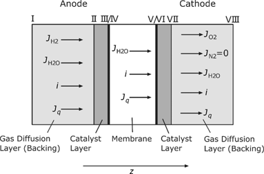
The CLs are considered as a microporous diffusion layer and an infinitesimal thin reaction layer. Figure 1 includes also the different fluxes across the fuel cell. In all bulk domains, electrical current j, heat Jq and amount of a substance Ji are transported. At the anode and at the cathode, a water flux JH2O besides the hydrogen flux JH2 and the oxygen flux JO2 is considered. This is also true for the electrolyte membrane.

Figure 1:

Schematic structure of the analyzed PEMFC.

Table 2 contains all the fluxes and their intrinsic corresponding forces according to Figure 1. They are only defined in the z-direction in accordance to our one-dimensional analysis. A negative flux indicates a transport opposite to the positive z-direction, as it is expected, e.g. for the oxygen flux at the cathode GDL.

Table 2:

Fluxes and corresponding forces in the different domains of the PEMFC.

Anode		Membrane		Cathode
Flux	Force	Flux	Force	Flux	Force
i	−1Tdϕdz	i	−1Tdϕdz	i	−1Tdϕdz
Jq	−1T2dTdz	Jq	−1T2dTdz	Jq	−1T2dTdz
JH2O	−1TdμH2O,Tdz	JH2O	−1TdμH2O,Tdz	JH2O	−1TdμH2O,Tdz
JH2	−1TdμH2,Tdz			JO2	−1TdμO2,Tdz

After evaluating eq. (4) with this set of forces and fluxes, we can calculate the volumetric entropy production σˆ in W/WKm3Km3 for all GDLs and for the electrolyte. For the anode-GDL (backing), the entropy production reduces to

(8)σˆAB=−JH2OT⋅dμH2O,Tdz−JH2T⋅dμH2,Tdz−JqT2⋅dTdz−iT⋅dϕdz

Respectively, for the cathode-GDL (backing), we have

(9)σˆCB=−JH2OT⋅dμH2O,Tdz−JO2T⋅dμO2,Tdz−JqT2⋅dTdz−iT⋅dϕdz

and for the membrane:

(10)σˆM=−JH2OT⋅dμH2O,Tdz−JqT2⋅dTdz−iT⋅dϕdz.

The entropy production at the catalyst surface is related to the overpotential given by the reaction kinetics. Due to the nature of the overpotential η, it can be interpreted as a thermodynamic force if it is divided by the absolute temperature, as it is the case for the other forces (see Table 2). The following relations are obtained for the area-specific entropy production rate ˙Sˆirr in W/m2K at the CLs for the anode (A) and the cathode (C):

(11)˙SˆirrA=i⋅ηAT

(12)˙SˆirrC=i⋅ηCT

This relationship can be also obtained straight forward with an energy and an entropy balance for the reaction layer. In this case, the lost power defined by the product of the electric current and the overpotential:

(13)Pˆloss=i⋅η

becomes a heat source ˙qˆloss, which is directly related to the entropy production ˙Sˆirr:

(14)˙Sˆirr=˙qˆlossT=i⋅ηT

This entropy production must be distinguished from the reaction entropy ΔrS on the anode and the cathode side, which is a reversible entropy term.

3 Modeling

As stated before, we will consider the GDL, the CL for both electrodes, respectively, and the electrolyte membrane in our one-dimensional model only. The CLs are divided in a microporous mesh and an infinitesimal thin reaction layer.

We will consider a steady-state situation and one-dimensional fluxes in the z-direction. The balance- and transport equations are solved simultaneously to calculate the temperature-, partial pressure- and voltage profiles as well as the molar- and heat fluxes. Subsequently, the equations for the entropy production rate are solved locally for every domain of the PEMFC. Ideal gas behavior is assumed to describe all gases and gas-mixtures, an incompressible fluid is assumed to describe all liquid phases.

As a first approximation, only the transport equations in the membrane are provided by the theory of non-equilibrium thermodynamics in this paper. The reason for this is that some of the forces and fluxes in the membrane are strongly coupled and can’t be neglected in the modeling approach. In contrast to the membrane, the other domains are modeled with not only conventional approaches like the Fourier’s law, but also with extended approaches for describing the coupling between some of the forces and fluxes like the Maxwell–Stefan equations [21]. The coupling effects in the domains, which are not considered, are less pronounced to our present knowledge.

3.1 Gas diffusion layer

The GDL allows for electric conduction between the bipolar plate and the CL. Furthermore, the reaction gases diffuse from the gas channel through the GDL to the CL. To take species and momentum transport into account, the mass transport in the porous solid can be described by the Dusty Gas Model. Multicomponent diffusion can be described by the Maxwell–Stefan equation [21]:

(15)−1RTdpidz=∑j=1NxjJi−xiJjDij

where Dij is the Maxwell–Stefan-diffusion coefficient, xi the mole fraction, pi the partial pressure and Ji the flux of component i. If the porous medium is considered as an additional component (N+1), made up of huge molecules and the flux of this component is set to zero (JN+1=0), eq. (15) can be written as

(16)−1RTdpidz=∑j=1Nx′jJi−x′iJjD′ij+x′N+1JiD′i,N+1

This approach makes it possible to consider collisions between the species and the solid phase. It is important to note here that the mole fractions and the diffusion coefficients are defined for the pseudo mixture. These diffusion coefficients can be expressed with the respective effective diffusion coefficient, i.e. Dije, the effective Maxwell–Stefan-diffusion coefficient and DiKn,e the effective Knudsen-diffusion coefficient as follows [23]:

(17)Dij′=cc′Dije

(18)Di,N+1′=xN+1′DijKn,e

(19)xi′=cc′xi

where c′ is the concentration in the pseudo mixture. Based on the insight that the diffusion takes place in the pores of the GDL only, the diffusion coefficients are corrected by the tortuosity τ and the porosity ε of the porous structure as follows:

(20)DiKn,e=ετDiKn

(21)Dije=ετDij

Whether the Maxwell–Stefan- or the Knudsen-diffusion dominates depends on the mean free path of the gas molecules and the pore size. In addition to the diffusion terms the convective transport must be considered. Finally, we obtain for the gradient of the partial pressure in the GDL [23]:

(22)−dpidz−B0piηvDiKn,edpdz=RTJiDiKn,e+∑j=1NxjJi−xiJjDije

The required Maxwell–Stefan diffusion coefficients are calculated by the correlation of Fuller [24]:

(23)Dij=1.013⋅10−2⋅T1.75(Mi+Mj)/MiMjp(νijD3+νjD3)2 [m2/s]

where νiD is the dimensionless diffusion volume (taken from [21]), Mi is the molar mass of the component ig/mol, T the temperature K and p the pressure Pa, respectively. The pores are considered to be cylindrical with a radius rp, so that the Knudsen diffusion coefficient is obtained from the kinetic theory of gases:

(24)DiKn=43⋅rp2RTπMi

The permeability B0 in the convective term within a porous structure follows by comparison with the Law of Hagen–Poiseuille:

(25)B0=ετ18rp2

Finally, the dynamic viscosity of the gas mixture ηv is determined with the pure-component viscosities ηv,i and the mixing rule of Herning [25]:

(26)ηv=∑i=1Nxiηv,i0Mi∑i=1NxiMi

For the calculation of the temperature-dependent pure-component viscosities, the recommended procedure from the VDI Heat Atlas [26] is used.

3.1.1 Anode GDL

As shown in Figure 1, the transport of hydrogen, water vapor, heat and electric current must be considered in the calculation of the anode GDL. Due to the steady-state condition, the component fluxes are constant. According to Faraday’s law, the hydrogen flux density can be obtained directly from the current density as follows:

(27)JH2=i2F

The water flux density cannot be calculated at the beginning of the iteration and has to be estimated. As it is usually done, we relate the water flux to the hydrogen flux by a proportionality factor β:

(28)JH2O=β⋅JH2

In the energy balance, the enthalpies of the mass fluxes, the heat transfer in the solid phase and the electric dissipation are considered. Due to the assumption of ideal gas behavior and constant molar heat capacities of the gases, the gradients in enthalpies are rewritten by the temperature gradients:

(29)dJqdz=−JH2⋅cp,H2dTdz−JH2O⋅cp,H2OdTdz−idϕdz

While the diffusion is modeled with the Dusty Gas Model, the heat transfer and the electric conduction is modeled by the Fourier’s- and the Ohm’s law. By introducing the thermal conductivity λth and the specific electrical resistance rel in the energy balance, the differential equation for the temperature profile is given by

(30)0=d2Tdz2−1λthJH2⋅cp,H2+JH2O⋅cp,H2OdTdz+i2relλth

3.1.2 Cathode GDL

In the cathode GDL, we consider the reactant oxygen, the product water and nitrogen as an inert gas. As already explained for the hydrogen flux, the oxygen flux density is related to the current density due to the stoichiometry:

(31)JO2=−12JH2=−i4F

The sign of the fluxes is determined by the definition of the z direction in space. Two different contributions to the water flux density on the cathode have to be considered: the water coming out of the electrolyte membrane and the reaction product at the cathode:

(32)JH2O=β+1⋅JH2

At steady state, the nitrogen flux density can be set to zero. Hence, the energy balance for the cathode can be rearranged to the following differential equation for the temperature:

(33)0=d2Tdz2−1λthJO2⋅cp,O2+JH2O⋅cp,H2OdTdz+i2relλth

3.2 Catalyst layer

The microporous structure of the CL is modeled as described in Section 3.1. Due to the higher density of the porous structure, we use different values for the tortuosity, the porosity and the radius of the pores as compared to the GDL. The impact on the heat conductivity and the specific electrical resistance is calculated as follows:

(34)λthCL=λthGDL1−εCL1−εGDL

(35)relCL=relGDL1−εGDL1−εCL

3.2.1 Anode catalyst layer

The calculation of the kinetics on the anode is based on the Tafel–Volmer Mechanism. According to [27–29], it can be assumed that the Tafel-step (hydrogen adsorption) is the rate limiting reaction step. With the surface coverage θ, which is the ratio of the occupied adsorption sites to the overall sites (0≤θ≤1), the current density can be calculated as follows:

(36)i=i01−θ1−θ02−θθ02

where θ0 is the equilibrium surface coverage for i=0 and i0 is the exchange current density. Following the approach of [30] and [29], the surface coverage can be calculated in terms of the overpotential ηA:

(37)θ=θ01−θ0 exp ηAFRT+θ0

Insertion of eq. (37) into eq. (36) yields the following expression:

(38)i=i01θ0+1−θ0expηAF/ηAFRTRT2exp2FηART−1

As reported in the literature [31, 32], the equilibrium surface coverage on platinum is above 0.9. Especially for small overpotentials, eq. (38) can be simplified:

(39)i=i0exp2FηART−1

It must be taken into consideration that the exchange current density refers to the surface of the catalyst and the current density refers to the entire cell area. To take this into account, a surface enlargement factor fV is introduced and a subsequent transformation of eq. (39) leads to the following equation for the overpotential at the anode:

(40)ηA=RT2Flnii0fV+1

The concentration dependency of the equilibrium exchange current density is usually described as follows (see [33–36]):

(41)i0=i0refpH2pH2ref0.5

where i0ref is the reference exchange current density.

In steady state, the mass balance at the reaction layer gives a constant water flux density. While the water in the GDL is gaseous, the water in the membrane is in an adsorbed state. In a first approximation, this condition can be modeled as a liquid phase. The hydrogen oxidizes completely to protons, no crossing is considered. In the energy balance, we replace the reaction enthalpy ΔrhA by the free reaction enthalpy ΔrgA and the reversible heat of reaction TΔrsA. The reaction Gibbs enthalpy is related to the reversible voltage and just the overpotential remains in the energy balance:

(42)JqIV=JqIII+T−ΔrsAJH2+ηA⋅i+ΔVh⋅JH2O

where ΔVh is the enthalpy of condensation.

3.2.2 Cathode catalyst layer

For the modeling of the electrode kinetics at the cathode, we use the Butler–Volmer equation:

(43)i=i0exp1−αnelFηCRT−expαnelFηCRT

We set the charge transfer coefficient α to 0.5 so that the overpotential can be calculated analytically:

(44)ηC=2RTnelFarcsinhi2i0fV

In most of the cases, the models in the literature differ in the reaction mechanism, which affects directly the number of exchanged electrons nel for one reaction step as well as the Tafel slope. In this study, we use two different reaction mechanisms depending on the overpotential. For small over potentials and high electrode potentials ΔϕC, a mechanism with 2 exchanged electrons is used. For small electrode potentials, a reaction mechanism with 1 exchanged electron is used:

(45)nel=2forΔϕK≥775mV

(46)nel=1forΔϕK<775mV

Compared to the anode, Paratharathy et al. [37] shows that the concentration dependency of the equilibrium exchange current density is a first order function:

(47)i0=i0refpO2pO2ref

At the cathode reaction layer, the oxygen reacts with the hydrogen protons to create water. Because of this, the water flux density changes as described in eq. (32). If the water at the cathode is modeled as a vapor phase, the energy balance is given by

(48)JqVI=JqV+T−ΔrsCJO2+ηC⋅i−ΔVh⋅JH2OV

3.3 Membrane

In the membrane, a water flux, the electric current and the heat flux are considered. Special attention should be devoted to the amount of water in the membrane, because of its impact on the electrical resistivity. Due to the absorbed water, the membrane swells and changes the size. The swelling of the membrane is proportional to the water content. This effect is considered with a swelling factor s (see Figure 2).

Figure 2:

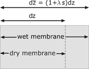
Volume element of the dry and wet membrane.

The water content λ is the molar ratio between the adsorbed water and the negative-charged sulfonic ions in the membrane:

(49)λ=nH2OnSO3−

It is typically calculated by means of adsorption isotherms. In this model, we apply the one suggested by Hinatsu et al. [38] at 80°C:

(50)λ=0.3+10.8⋅aH2O−16⋅aH2O2+14.1⋅aH2O3

We approximate the activity close to the reaction layers with the partial pressure and the vapor pressure:

(51)aH2O=pH2OpH2OsT

The vapor pressure is calculated with the Wagner approximation [39]. The kinetics is described in means of linear non-equilibrium thermodynamics. The phenomenological equations following from Table 2 are given by

(52)Jq=−LqqT2dTdz˜−LqwTdμH2O,Tdz˜−LqϕTdϕdz˜

(53)JH2O=−LwqT2dTdz˜−LwwTdμH2O,Tdz˜−LwϕTdϕdz˜

(54)i=−LϕqT2dTdz˜−LϕwTdμH2O,Tdz˜−LϕϕTdϕdz˜

After solving eq. (54) for the gradient in the electrical potential, it can be replaced in eqs. (53) and (52). Thereby, the heat flux density is given by the following expression:

(55)Jq=−λthdTdz˜−lqwdμH2O,Tdz˜+πi

where by algebraic rearrangement:

(56)λth=LqqT2−LqϕLϕqLϕϕT2

(57)lqw=LqwT−LqϕLϕwTLϕϕ

(58)π=LqϕLϕϕ

Similarly, the water flux density can be obtained as

(59)JH2O=−lwqTdTdz˜−lwwdμH2O,Tdz˜+tH2OFi

where

(60)lwq=LwqT−LwϕLϕqTLϕϕ

(61)lww=LwwT−LwϕLϕwTLϕϕ

(62)tH2O=FLwϕLϕϕ

Introducing the Onsager reciprocal relations, the electrical current can be simplified to

(63)i=−πκTdTdz˜−tH2OκFdμH2O,Tdz˜−κdϕdz˜

with

(64)κ=LϕϕT

In this model, the thermal diffusive (Soret/Dufour effect) and thermal electric effects (Peltier/Seebeck effect) in the membrane are neglected as a first approximation. The only coupling effect which is considered is the electroosmotic water transport and its counterpart. Under these conditions, the water flux density can be simplified to give

(65)JH2O=−lwwdμH2O,Tdz˜+tH2OFi

As reported in the literature [5, 40], the coefficient lww can be approximated as follows:

(66)lww=DH2OcH2ORT

where cH2O is the molar water concentration:

(67)cH2O=λρtrXtr1+sλ

Here, ρtr is the dry membrane density, Xtr the amount of SO3− moles divided through the mass of the dry membrane and 1+sλ the swelling factor. In this work, it is assumed that the water in the membrane is in chemical equilibrium with the surrounding gas. In this case, the gradient in chemical potential at constant temperature can be written in terms of the water content and the activity as follows:

(68)dμH2O,Tdz˜=RTdlnaH2Odz˜=RT1aH2OdaH2Odλdλdz˜

where

(69)μH2O,T=μH2O0+RTlnaH2O

By introducing eqs. (66)–(68) and JH2O=β⋅i/2F into eq. (65) and after a coordinate transformation to the coordinate of the dry membrane, the differential equation of the water content becomes

(70)dλdz=2tH2O−β2F⋅i⋅DH2O⋅λ⋅ρtr⋅Xtr1+sλ21aH2OdaH2Odλ−1

To solve this equation, the inverse function of eq. (50) aH2O=aH2Oλ is necessary. This inverse function is approximated numerically with the software Maple [41]. We then have valid in the range of 0≤λ≤9:

(71)aH2O=10−93c−0.3367109c+0.3783

where

(72)c=−2.7373⋅1027+9.5745⋅1026⋅λ+3⋅108⋅9.4710⋅1037−5.8241⋅1037⋅λ+1.0186⋅1037⋅λ21/3

The derivation of the activity with respect to the water content [see eq. (50)) is finally calculated given by following expression:

(73)daH2Odλ=(dλdaH2O)−1=(10.8−32.0⋅aH2O+42.3⋅aH2O2)−1

Taking into consideration the ohmic conduction and the electroosmotic coupling effect the gradient of the electric potential can be calculated as follows:

(74)dϕdz˜=−tH2OFdμH2O,Tdz˜−iκ

With eq. (68) and a coordinate transformation to the coordinate system of the dry membrane, the final equation for the electric potential in our model becomes

(75)dϕdz=−tH2OFRTaH2OdaH2Odλdλdz−iκ1+sλ

As already discussed for the GDL the temperature gradient is obtained from an energy balance. In the membrane the electric dissipation, the heat transfer and the enthalpy of the water flux are considered. Because of the typically small temperature difference a constant heat capacity is assumed

(76)dJqdz˜=−JH2O⋅cp,H2OdTdz˜+idϕdz˜

If coupling effects are neglected, the heat flux can be described by the Fourier’s law:

(77)Jq=−λthdTdz˜

By introducing the Fourier’s law and transforming the coordinate system in eq. (76), the temperature gradient can be calculated by the following differential equation:

(78)d2Tdz2=1+sλ2λthJH2O⋅cp.H2O11+sλdTdz−i⋅11+sλdϕdz

3.3.1 Transport coefficients

An important issue is the assumption for the description of the transport coefficients. According to Neubrand [40], the heat conductivity of the Nafion membrane can be set to a constant value:

(79)λth=0.43 [W/m K]

In this study, we propose the following relationship between the self-diffusion coefficient at 303K and the water content based on the experimental results of Zawodzinski et al. [42]:

(80)DH2O303 K=51+(4.47/λ)2.85⋅10−10 [m2/s]

Due to the different operation temperature, the diffusion coefficient has to be corrected by an Arrhenius approach as stated by Springer et al. [5]. Our approach is based on measurements of Yeo et al. [43]:

(81)DH2O=DH2O303K⋅exp2416K1303K−1T

Different equations for the transport number have been proposed in the literature. In this work, the empirical correlation of Springer et al. [5] is used:

(82)tH2O=2.5⋅λ22.

As already mentioned, the proton conductivity in Nafion is a function of the water content and the temperature. To take this into account, an empirical correlation of Springer et al. [5] is used:

(83)κ=0.5139⋅λ−0.362⋅exp1268K1303K−1T

3.4 Overall model

For the calculation of the described domains, boundary conditions for the electric current, the temperature and the composition of the supplied gases are necessary. Figure 3 illustrates the supply channels and the boundary of the model cell.

Figure 3:

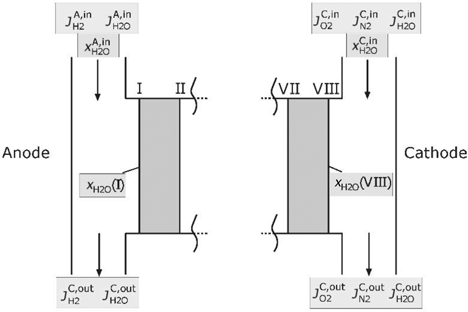
Supply channels of the PEMFC.

The temperature in the supply channel will be assumed as T(I). If the hydrogen in the inlet at the anode side is saturated with water, the mole fraction may be written as follows:

(84)xH2OA,in=pH2OspA

With a given stoichiometric factor νH2, the consumed hydrogen flux, the hydrogen and water fluxes as well as the concentration at the inlet (A, in), at position (I) and at the outlet (A, out) of the anode are related by the following equation set:

(85)JH2A,in=νH2⋅JH2I

(86)JH2OA,in=xH2OA,in⋅JH2A,in1−xH2OA,in

(87)JH2A,out=JH2A,in−JH2I

(88)JH2OA,out=JH2OA,in−JH2OI

(89)xH2OA,out=JH2OA,outJH2OA,out+JH2A,out

(90)xH2OI=xH2OA,in+xH2OA,out2

The partial pressure of water on the cathode will be calculated in a different way. Similar to the literature [7, 32, 44], it is assumed that the membrane is fully hydrated on the cathode side. The partial pressure pH2OVIII on the border of the cathode GDL will be iterated until this condition is fulfilled.

4 Results and discussion

For the calculation of the balance- and transport equations, a FORTRAN 95 code is written. The differential equations are solved with the software packages NAG FORTRAN 77 which includes the routines D02PCV and DO2PVF. These routines can solve first-order differential equations with the Runge–Kutta method. Because of this, the second-order differential equations are transferred to a first-order system by substitution.

4.1 Current–voltage characteristic

The polarization curve obtained from the simulation model together with experimental data of Meier [45] is shown in Figure 4. In this case, the cathode gas was simulated with pure oxygen. A good agreement between the measured and the calculated voltage can be observed. At medium current, densities are the maximum deviation 10%.

$Figure 4: Simulated polarization curve together experimental data of Meier [40], H2/O2-cell, Nafion 117, T=80°C, pA= pK=2 bar, νH2=1${\nu _{{{\rm{H}}_{\rm{2}}}}} = 1$.$

Figure 4:

Simulated polarization curve together experimental data of Meier [40], H₂/O₂-cell, Nafion 117, T=80°C, p_A= p_K=2 bar, νH2=1.

$Figure 5: Simulated polarization curve together with simulation results of Meier [40], H2/Air-cell, Nafion 117, T=80°C, pA=pK=2 bar, νH2=1.5${\nu _{{{\rm{H}}_{\rm{2}}}}} = 1.5$.$

Figure 5:

Simulated polarization curve together with simulation results of Meier [40], H₂/Air-cell, Nafion 117, T=80°C, p_A=p_K=2 bar, νH2=1.5.

Usually, the oxygen in PEMFC’s is supplied by an air stream, so from now on the cathode gas is simulated with air. As shown in Figure 5, the voltage decreases at medium current densities more than in the simulation results of Meier [45]. The main reason for this is the adsorption isotherm of Springer used by Meier which has a maximum water content of λ≈14. In contrast, the used adsorption isotherm of Hinatsu, which is valid for a temperature of 80°C, has a maximum water content of λ≈9. This leads to a lower electric conductivity.

For Figure 5 and the following simulation results, the boundary conditions

(91)pI=pVIII=2bar

(92)TI=TVIII=80∘C

as well as the stoichiometric factor νH2=1.5 are used. The other coefficients are reported in Table 3.

Table 3:

Parameters for simulation.

Property	Sign	Value	Source
Gas diffusion layer (backing)
Thickness	d	180×10−6m	[7, 32]
Radius of the pores	rp	10×10−6m	[32, 45]
Porosity	ε	0.4	[32, 45]
Tortuosity	τ	2.6	[32, 45]
Thermal conductivity	λth	15.6W/mK	[32, 46]
Specific electrical resistance	rel	5×10−3Ωm	[31]
Porous catalyst layer
Thickness	d	10×10−6m	[7, 45]
Radius of the pores	rp	50×10−9m	[32, 45]
Porosity	ε	0.07	[32]
Tortuosity	τ	5	[32]
Thermal conductivity	λth	Eq. (34)	–
Specific electrical resistance	rel	Eq. (35)	–
Anode reaction layer
Reference exchange current density	i0ref	8A/m2	[45]
Reference partial pressure	pH2ref	1bar	[45]
Surface enlargement factor	fV	200	[45]
Molar reaction entropy	Δrs	−130.68J/molK	–
Cathode reaction layer
Reference exchange current density	i0ref	1.44×10−4A/m2	[37]
Reference partial pressure	pO2ref	1.11458bar	[37]
Surface enlargement factor	fV	200	[45]
Molar reaction entropy	Δrs	−65.32J/molK	–
Membrane
Thickness (dry)	d	175×10−6m	[5, 45]
Ion exchange capacity (dry)	Xtr	0.909mmol/g	[5, 40]
Density (dry)	ρtr	2050kg/m3	[40]
Thermal conductivity	λth	0.43W/mK	[40]
Swelling factor	s	0.0123	[5, 40]

4.2 Local field quantities

4.2.1 Membrane water content

The water content in the Nafion-membrane is an important parameter because it is directly related to the electrical conductivity. A local dehydration leads e.g. to high power losses. The calculated water content as a function of the current density and the z-coordinate is shown in Figure 6. 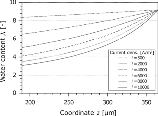Because of the assumption of a gas phase at the cathode electrode which is saturated with water, the water content reaches the maximum of λ≈9 at the cathode. For low current densities, the value on the anode is slightly lower. With higher current densities, the water content decreases faster. Because of the coupled transport processes, the dehydration takes place in a wide range of the membrane. The shape of the curve can be described as convex. Many studies in the literature come to similar results [5, 45, 47–49], but in some others, a linear [50] or a concave curve [51, 52] of the water content is reported.

Figure 6:

Water content in the Nafion membrane at different current densities.

Figure 7:

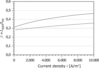
Proportionality factor as a function of the current density.

Figure 7 shows the simulation results of the proportionality factor as a function of the current density. For comparison, the simulation results of Meier [45] are indicated by the dashed curve. Springer [5] and Jansen et al. [53] estimated experimentally a relative water transport of β=0.4 at a current density of i=5,000A/m2, which fits very well to the simulation data presented here.

4.2.2 Electric potential

The characteristic curve of the electric potential as a function of the current density and the coordinate z is shown in Figure 8. At the border of the anode GDL, the electric potential is arbitrarily set to zero. This means the electric potential at the end of the cathode GDL is equal to the cell voltage. As reported before, the cell voltage decreases significantly with increasing current density. This results mainly from the ohmic losses in the membrane. Because of the dehydration effects and the resulting change of the electric resistivity, the potential drop is disproportionate to the current density. As already seen in Figure 6, the dehydration takes place at the anode side. This leads to a high voltage drop at the anode side of the membrane. On the other hand, the ohmic losses in the GDLs are very low.

Figure 8:

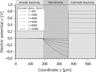
Electric potential in the PEMFC at different current densities.

4.2.3 Temperature

In this study, we assumed the temperature on the boundaries of the cell to be equal and to be held constant. This calls for a heat flux across both boundaries. Because of the irreversible processes, dissipative heat is released and the temperature increases. The temperature profile which arises for different current densities is shown in Figure 9. For low current densities, the cell behaves nearly isothermal. At high current densities, the temperature in the GDLs rises linearly. The released internal heat yields to a temperature maximum in the middle of the membrane which is slightly shifted to the anode side. This is due to the lower water content and the reduced electrical conductivity in this region.

Figure 9:

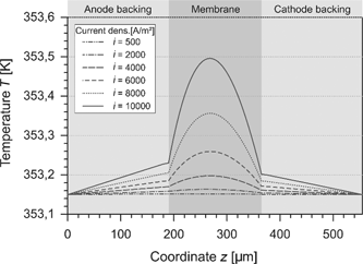
Temperature in the PEMFC at different current densities.

The temperature at the anode CL is above the temperature of the cathode CL. Initially, it seems to be wrong because the electrochemical irreversibility at the cathode is higher than at the anode. Nevertheless, the heat of reaction and the heat of condensation have to be considered. As described in eqs. (42) and (48), the released heat comprises different parts. These parts can be divided in a reversible and an irreversible part:

(93)Jq∗=T−ΔrsJH2/O2±ΔVh⋅JH2O⏟reversible+ηA/C⋅i⏟irreversible

The different values for a current density of i=8,000A/m2 are shown in Table 4. It follows that the released heat in the anode is higher because of the reversible part. Measurements of Vie [50] support the higher temperature at the anode.

Table 4:

Released heat in the catalyst layers.

	i=8,000A/m2
	Anode	Cathode
η	0.0239V	0.4552V
Jq,rev∗	2,691W/m2	−2,023W/m2
Jq,irr∗	191W/m2	3,642W/m2
Jq∗	2,882W/m2	1,619W/m2

4.2.4 Partial pressure in diffusion layer

4.2.4.1 Anode

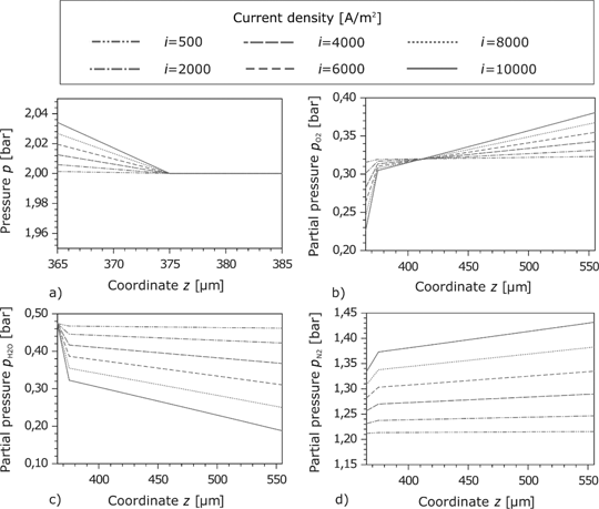
The pressure in the anode GDL is nearly constant due to the high porosity. In the CL, the pressure drop is higher which results from the denser pores structure. As expected, the pressure drop rises with the current density. Within the GDL, the partial pressure of H2 and H2O are nearly constant, only a small enrichment of H2 can be located which is also described in [5, 54]. At high current densities, the partial pressures decrease in the CL. A stoichiometric hydrogen supply at high current densities leads to a higher H2 partial pressure. Accordingly, a decrease in the H2O partial pressure can be observed, which causes the dehydration in the membrane because of the higher water transport.

Figure 10:

Pressure in the cathode GDL and the porous reaction layer at different current densities.

4.2.4.2 Cathode

The pressure profiles at the cathode GDL and the CL are similar to those at the anode side in the sense that the higher pressure drop is located at the CL (here at z<375μm) and not at the GDL (z>375μm). The pressure decreases toward the gas channel because the main stream flows also in this direction (Figure 10(a)).

The oxygen flows in the negative direction of the z-axis to the CL. In this direction, its partial pressure decreases. Due to the pressure drop at high current densities, the exchange current density decreases and the overpotential increases. At the boundary of the cathode feed channel, the oxygen partial pressure rises with the current density (Figure 10(b)). The opposite effect is observed by the water partial pressure. A large gradient of pH2O is necessary to ensure the removal of the produced water and maintain the fully hydrated condition in the membrane (Figure 10(c)). For the sake of completeness, Figure 10(d) shows the partial pressure of nitrogen. Despite no nitrogen flow in the stationary state, the partial pressure increases from the membrane to the feed channel.

4.3 Entropy production rate

4.3.1 Membrane

The overall entropy production rate must be positive but a single part can also be negative. According to eq. (10), the entropy production rate in the membrane results from three parts:

(94)σˆH2O=−JH2O1TdμH2O,Tdz

(95)σˆq=−Jq1T2dTdz

(96)σˆϕ=−i1Tdϕdz

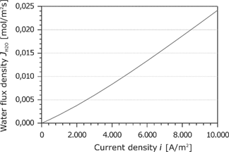
Due to the mass balance, the water flux in the membrane is constant. Figure 11 shows the water flux as a function of the current density. The water flux increases slightly and flows always toward the cathode. This is because the electroosmotic transport is larger than the back diffusion. The following entropy production rate σˆH2O is shown in Figure 12. At low current densities, the entropy production is nearly constant but for higher current densities, it increases because of the rising thermodynamic force and the inhomogeneous hydration of the membrane. It can be noticed that the value is negative. The reason for this is that the chemical potential of water rises with the water content toward the positive z-coordinate. According to this, the thermodynamic force is negative.

Figure 11:

Water flux density in the membrane as a function of the current density.

Figure 12:

Entropy production rate caused by the water flux in the membrane for different current densities.

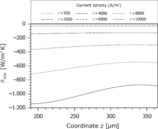
The heat flux in the membrane is shown in Figure 13. Because of the dissipative effects, it changes locally. As can be seen in the temperature profile (see Figure 9), the temperature gradient is zero in the middle of the membrane. At this point, the heat flux changes the direction. Furthermore, there is a large increase with the current density. The concave curve results from the fact that the values refer to the dry membrane.

Figure 13:

Heat flux density in the membrane for different current densities.

Figure 14:

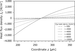
Entropy production rate caused by the heat flux in the membrane for different current densities.

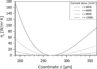
Due to the same sign of the thermodynamic force and its corresponding flux, the entropy production rate is always positive (see Figure 14). The entropy production rises exponentially with the current density.

Figure 15:

Entropy production rate caused by the current density.

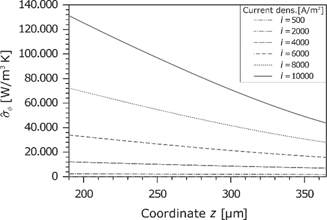
The last contribution to the entropy production rate in the membrane is due to the ohmic losses. As described before, the electric potential drop increases with the current density and the gradient at the anode is higher because of the lower water content. This effect can be directly transferred to the entropy production rate (see Figure 15). The contribution to the overall entropy production rate is always positive because the electric current flows in the direction of the negative potential gradient. Particularly, the inhomogeneous hydration leads to a high dissipation. Basically, the entropy production due to the ohmic losses is the most significant part.

Figure 16:

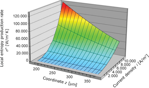
Overall entropy production rate as a function of the z-coordinate in the membrane and the current density.

Figure 16 shows the overall entropy production rate as a function of the z-coordinate and the current density. At low current densities, the dissipation in all regions of the membrane is very small, but for high current densities, it rises especially at the anode site.

4.3.2 Gas diffusion layer

The considered region of the anode and cathode side consists of the GDL and the microporous structure of the reaction layer. As described for the membrane, the overall entropy production rate can be separated in three parts.

The dissipation due to the material transport includes every substance flux and their corresponding forces:

(97)σˆST=JH2⋅XH2+JH2O⋅XH2OAnode

(98)σˆST=JO2⋅XO2+JH2O⋅XH2OCathode

For the calculation of the forces, respectively, the chemical potentials of the species are needed:

(99)μi=μi0+RTlnpip0

(100)dμi,Tdz=RTp0pidpi/pip0p0dz

The thermodynamic forces can be calculated knowing the partial pressure and temperature profiles. The entropy production rate for the anode and cathode is shown in Figure 17. Due to the denser structure, the dissipation in the microporous part is significantly higher.

Figure 17:

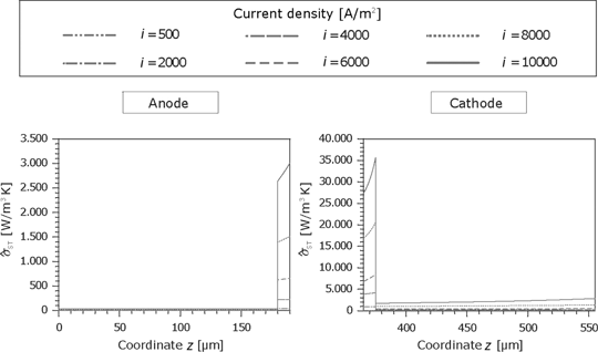
Entropy production rate caused by the substances fluxes in the GDL and the porous reaction layer for the anode and cathode side.

In contrast to the membrane, the heat flux in the GDL is nearly constant but increases with the current. As shown in Figure 18, the anode heat flux is higher than the cathode heat flux and the thermodynamic forces in the microporous layers are smaller because of the better heat conductivity. Accordingly, the dissipation is also lower in this region.

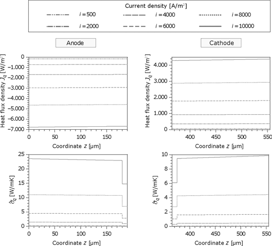
Figure 19 shows the corresponding force of the electric current and the resulting entropy production rate at the anode. Because of the same material properties and small temperature gradients, the results for the cathode are identical. The corresponding force Xϕ rises proportional and the entropy production rate σˆϕ disproportionately with the current density.

Figure 18:

Heat flux and the entropy production rate in the GDL and porous reaction layer for the anode and cathode side.

Figure 19:

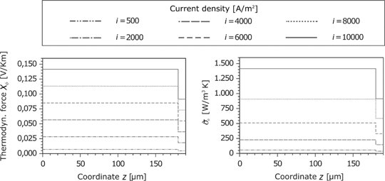
Thermodynamic force and entropy production rate caused by the current density in the GDL and the porous reaction layer for the anode.

Figure 20:

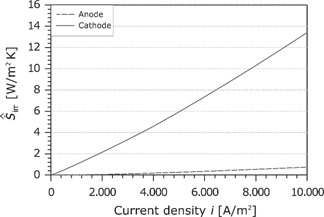
Area-specific entropy production rate in the anode and cathode CL as a function of the current density.

4.3.3 Area-specific entropy production rate

The entropy production rates described in the previous section are volumetric values. In order to compare the losses in the infinitesimal reaction layers with the losses in the volumetric domains, an area-specific entropy production rate is introduced.

(101)˙Sˆirr=∫0Lσˆdz

4.3.3.1 Catalyst layer

As already seen in eqs. (11) and (12), the intrinsic corresponding force of the current density in the electrode is

(102)Xη=ηT

The area-specific entropy production rate follows from the product of the corresponding force and the flux (see Figure 20). Similar to the overpotential, the entropy production rate increases slightly with the current density.

Figure 21:

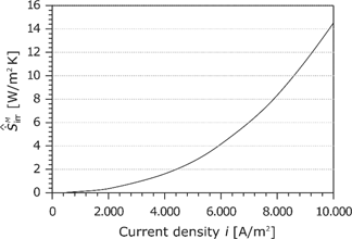
Area-specific entropy production rate in the membrane as a function of the current density.

4.3.3.2 Membrane

The area-specific entropy production rate ˙SˆirrM covers all irreversible processes:

(103)˙SˆirrM=∫z=190μmz=365μmσˆϕ+σˆq+σˆH2Odz

At high current densities, the losses in the membrane have the same order of magnitude as the cathode losses (see Figure 21).

Figure 22:

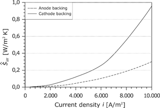
Area-specific entropy production rate in the GDL as a function of the current density.

4.3.3.3 Gas diffusion layers

As already done for the membrane, the losses in the GDLs are summarized in the area-specific entropy production rate:

(104)˙SˆirrAB,CB=∫dAB,CBσˆϕ+σˆq+σˆSTdz

As shown in Figure 22, the losses in the GDL are distinctly lower than the losses in the membrane and the cathode electrode.

4.3.3.4 Loss analysis

Besides the reversible heat release by the reaction entropy, the irreversibilities of the transport processes and electrode reactions are considered. This approach of the non-equilibrium thermodynamics to describe the losses of a fuel cell based on the explicit calculation of the entropy production rates differs from the conventional approach. These two approaches will be compared now for an exemplary current density of i=8,000A/m2.

Table 5:

Area-specific entropy production rate for i=8,000A/m2. The share gives the procentual contribution to the total entropy production rate.

Domain	Sign	Value W/m2K	Share %
Anode CL	˙SˆirrA	0.541	2.71
Cathode CL	˙SˆirrC	10.312	51.72
Membrane	˙SˆirrM	8.342	41.83
Anode GDL	˙SˆirrAB	0.188	0.94
Cathode GDL	˙SˆirrCB	0.557	2.8

The overall area-specific entropy production rate becomes

(105)˙Sˆirrges=˙SˆirrA+˙SˆirrC+˙SˆirrM+˙SˆirrAB+˙SˆirrCB

With the values of Table 5, it follows for the example

(106)˙Sˆirrges=19.94W/m2K

Under the assumption of a constant ambient temperature TU=298.15K, the area-specific exergy loss is given by

(107)˙EˆxV=TU˙Sˆirrges=5945W/m2

In the conventional method, the overpotentials of the electrodes and the ohmic losses in the membrane and the GDLs will be added up. The overall voltage drop can be calculated with the values of Table 6 as

(108)Δϕges=ηA+ηC+ΔϕΩM+ΔϕΩAB+ΔϕΩCB=0.866V

Normally, the losses will be given as an area-specific electric power:

(109)PˆV=Δϕges⋅i=6,928W/m2

The voltage drop leads to a heat release and the calculated power loss is equal to this heat flux. Since the heat flux is not released at the ambient temperature, a certain exergy amount is included in it. The real area-specific exergy loss can be calculated with the assumption that the heat is released at the cell temperature T=353.15K:

(110)˙EˆxV=1−TUT⋅PˆV=5,849W/m2

The value is slightly below the result of the entropy calculation. This is mainly due to the fact that the substance transport losses in the GDLs are neglected.

If these contribution is also neglected for the calculation of ˙Sˆirrges is the deviation between the two results below 0.2%.

Table 6:

Overpotentials and ohmic losses for i=8,000A/m2. The share gives the procentual contribution to the sum of total overpotential and ohmic losses.

Domain	Sign	Value V	Share %
Anode CL	ηA	0.024	2.8
Cathode CL	ηC	0.455	52.5
Membrane	ΔϕΩM	0.373	43.1
Anode GDL	ΔϕΩAB	0.007	0.8
Cathode GDL	ΔϕΩCB	0.007	0.8

5 Conclusion

In this study, a thermo-electrochemical model for the simulation of the current–voltage characteristics and the irreversibilities in a PEMFC is developed and validated with experimental data. Based on the non-equilibrium thermodynamics, the local entropy production rate is calculated and the loss mechanisms can be quantified in a consistent thermodynamic way.

The fluxes needed and their intrinsic corresponding forces are calculated in a one-dimensional steady-state model. This model solves the balance and transport equations in every domain of the cell. Because of the strong coupling effects in the membrane, the transport equations in these domains are provided by the theory of non-equilibrium thermodynamics. In this way, the most important coupling effects can be considered directly.

For the description of the electrode processes, the current/overpotential relations are presented. In contrast to most literature approaches, the Nernst part, which is caused by concentration changes in the GDL, is not considered in the overpotential calculation because it is, in thermodynamic sense, no driving force for the electrode reaction. But the resulting irreversibilities are considered in the calculation of the entropy production rate. The calculated current–voltage characteristic is in good agreement with experimental data from the literature.

At high current densities, the increasing electroosmotic transport of water leads to a dehydration of the membrane at the anode side. The reduced electric conductivity in the membrane results in a strong increase of the entropy production rate. The irreversibilities at the cathode CL and the ones in the membrane lead to 93.5% of the entropy production in the cell. While the entropy production rate in the anode GDL is very small, the entropy production rate in the cathode GDL is comparable with the entropy production rate at the anode CL.

The presented thermodynamic analysis can be transferred to other electrochemical systems like electrolysis cells or other fuel cell types. It will be extended in future to discuss all the coupling effects which have been neglected in this paper. We thank S. Kjelstrup for helpful discussions.

Nomenclature

Latin letters

Symbol	Unit	Quantity
a	–	Activity of component i
Ar	J/mol	Affinity of reaction
B0	m²	Permeability
c	mol/m³	Concentration
cp	J/mol/K	Molar isobaric heat capacity
d	m	Thickness
Di	m²/s	Self-diffusion coefficient
Dije	m²/s	Effective Maxwell–Stefan-diffusion coefficient
DiKn,e	m²/s	Effective Knudsen-diffusion coefficient
EˆxV.	W/m²	Area-specific exergy loss
fV	–	Surface enlargement factor
Δrg	J/mol	Molar free reaction enthalpy
ΔVh	J/mol	Molar enthalpy of condensation
Δrh	J/mol	Molar reaction enthalpy
i	A/m²	Current density
i0	A/m²	Exchange current density
Ji	mol/m²s	Molar flux density of component i
Jq	W/m²	Heat flux density
K	–	Number of transport processes
lij		Modified phenomenological coefficient
Lij		Phenomenological coefficient
Mi	kg/mol	Molar mass
N	–	Number of components
n	mol	Amount of substance
nel	–	Number of electrons
p	Pa	Pressure
pi	Pa	Partial pressure of component i
Pˆ	W/m²	Area-specific electric power
˙qˆ	W/m²	Area-specific heat source
rel	Ω m	Specific electrical resistance
s	–	Swelling factor
˙Sˆirr	W/K	Area-specific entropy production rate
Δrs	J/mol K	Molar reaction entropy
ΔrS	J/K	Reaction entropy
tH2O	–	Transport number of water
T	K	Temperature
U	V	Cell voltage
x	–	Mole fraction
z	m	Membrane coordinate z (dry)
z˜	m	Membrane coordinate z (wet)

Greek letters

Symbol	Unit	Quantity
α	–	Charge transfer coefficient
β	–	Proportionality factor
ε	–	Porosity
ηv	kg/ms	Dynamic viscosity
η	V	Overpotential
θ	–	Surface coverage
κ	S/m	Specific electric conductivity
λ	–	Water content
th	W/m K	Thermal conductivity
μi	J/mol	Chemical potential of component i
˙ξr	mol/s	Reaction rate
π	V	Peltier coefficient
σˆ	W/m³ K	Volumetric entropy production rate
τ	–	Tortuosity
ϕ	V	Electric potential

References

[1] B. S. Pivovar, An overview of electro-osmosis in fuel cell polymer electrolytes, Polymer 47 (May 2006), no. 11, 4194–4202.10.1016/j.polymer.2006.02.071Search in Google Scholar

[2] G. Karimi and X. Li, Electroosmotic flow through polymer electrolyte membranes in PEM fuel cells, J. Power Sour. 140 (August 2004), no. 1, 10.10.1016/j.jpowsour.2004.08.018Search in Google Scholar

[3] C. Siegel, Review of computational heat and mass transfer modeling in polymer-electrolyte-membrane (PEM) fuel cells, Energy 33 (September 2008), no. 9, 1331–1352.10.1016/j.energy.2008.04.015Search in Google Scholar

[4] A. Z. Weber and J. Newman, Modeling transport in polymer-electrolyte fuel cells, Chem. Rev. 104 (August 2004), 4679–4726.10.1021/cr020729lSearch in Google Scholar

[5] T. E. Springer, T. A. Zawodzinski and S. Gottesfeld, Polymer electrolyte fuel cell model, J. Electrochem. Soc 138 (1991), no. 8, 2334–2342.10.1149/1.2085971Search in Google Scholar

[6] R. Mosdale and S. Srinivasan, Analysis of performance and of water and thermal management in proton exchange membrane fuel cells, Electrochim. Acta 40 (March 2000), no. 4, 413–421.10.1016/0013-4686(94)00289-DSearch in Google Scholar

[7] A. Rowe and L. Xianguo, Mathematical modeling of proton exchange membrane fuel cells, J. Power Sour. 102 (2001), no. 1–2, 82–96.10.1016/S0378-7753(01)00798-4Search in Google Scholar

[8] D. Singh, D. M. Lu and N. Djilali, A two-dimensional analysis of mass transport in proton exchange membrane fuel cells, Int. J. Eng. Sci. 37 (March 1999), no. 4, 431–452.10.1016/S0020-7225(98)00079-2Search in Google Scholar

[9] J. J. Basschuk and X. Li, Modelling of polymer electrolyte membrane fuel cells with variable degrees of water flooding, J. Power Sour. 86 (March 2000), no. 1–2, 181–196.10.1016/S0378-7753(99)00426-7Search in Google Scholar

[10] L. Onsager, Reciprocal relations in irreversible processes. I., Phys. Rev. 37 (February 1931), 405.10.1103/PhysRev.37.405Search in Google Scholar

[11] G. Klein and I. Prigogine, sur la mécanioue statistique des phénomènes irreversibles I, Phys. A: Stat. Mech. Appl. 19 (1953), no. 1–12, 74–88.10.1016/S0031-8914(53)80008-XSearch in Google Scholar

[12] K. Wagner and K. W. Hoffmann, Chemical reactions in endoreversible thermodynamics, Eur. J. Phys. 37 (2016), 1–10.10.1088/0143-0807/37/1/015101Search in Google Scholar

[13] K. Wagner and K. H. Hoffmann, Endoreversible modeling of a PEM fuel cell, J. Non-Equilib. Thermodyn. 40 (2015), no. 4, 283–294.10.1515/jnet-2015-0061Search in Google Scholar

[14] M. Wöhr and W. Neubrand, Dynamische simulation einer polymer-membran-brennstoffzelle (PEFC), Chem. Ing. Tech. 7 (1996), 842–845.10.1002/cite.330680718Search in Google Scholar

[15] S. Kjelstrup and A. Røsjorde, Local and total entropy production and heat and water fluxes in a one-dimensional polymer electrolyte fuel cell, J. Phys. Chem. B 109 (April 2005), no. 18, 9020–9033.10.1021/jp040608kSearch in Google Scholar PubMed

[16] K. S. Forland, T. Forland and S. K. Ratkje, Irreversible Thermodynamics – Theory and Applications, John Wiley, New York, 1988.Search in Google Scholar

[17] J. Schnakenberg, Vorlesungsskript Irreversible Thermodynamik Wintersemester 1994/95/Rheinisch Westfälische Technische Hochschule Aachen, 1994.Search in Google Scholar

[18] B. Hafskjold, T. Ikeshoji and S. K. Ratkje, On the molecular mechanism of thermal diffusion in liquids, Mol. Phys. 80 (April 1993), no. 6, 1389–1412.10.1080/00268979300103101Search in Google Scholar

[19] G. Lebon, Heat conduction at micro and nanoscales: A review throgh the prism of extended irreversible thermodynamics, J. Non-Equilib. Thermodyn. 39 (2014), no. 1, 35–59.10.1515/jnetdy-2013-0029Search in Google Scholar

[20] S. Bargmann, Remarks on the Green–Naghdi theory of heat conduction, J. Non-Equilib. Thermodyn. 38 (2013), no. 2, 101–118.10.1515/jnetdy-2012-0015Search in Google Scholar

[21] R. Taylor and R. Krishna, Multicomponent Mass Transfer, Wiley, New York, 1993.Search in Google Scholar

[22] J. A. Manzanares, M. Jokinen and J. Cervera, On the different formalisms for the transport equations of thermoelectricity: A review, J. Non-Equilib. Thermodyn. 30 (2015), no. 3, 211–227.10.1515/jnet-2015-0026Search in Google Scholar

[23] R. Jackson, Transport in Porous Catalysts, Elsevier, New York, 1977.Search in Google Scholar

[24] E. N. Fuller, P. D. Schettler and J. Giddings, A new method for prediction of binary gas-phase diffusion coefficients, Ind. Eng. Chem. 58 (1966), 19–27.10.1021/ie50677a007Search in Google Scholar

[25] R. C. Reid, J. M. Prausnitz and B. E. Poling, The Properties of Gases and Liquids, McGraw-Hill, New York, 1988.Search in Google Scholar

[26] VDI e.V, VDI-Wärmeatlas, Auflage 10, Springer Vieweg, Berlin-Heidelberg, 2006.Search in Google Scholar

[27] P. Ross, Electrode surface science: a physical basis for understanding the hydrogen and oxygen reaction on Pt group metal Electrode surfaces, in: Proceedings of the Workshop on the Electrocatalysis of Fuel Cell Reactions, The Electrochemical Society, New York (1978), 79–82.Search in Google Scholar

[28] P. Stonehart and P. N. Ross, The use of porous electrodes to obtain kinetic rate constants for rapid reactions and adsorption isotherms of poisons, Electrochim. Acta 21 (1976), 441–445.10.1016/0013-4686(76)85123-7Search in Google Scholar

[29] W. Vogel, J. Lundquist, P. Ross and P. Stonehart, Reaction pathways and poisons – II. The rate controlling step for electrochemical oxidation of hydrogen on Pt in acid and poisoning of the reaction by CO, Electrochim. Acta 20 (1975), 79–93.10.1016/0013-4686(75)85048-1Search in Google Scholar

[30] M. W. Breiter, Reaction mechanism of the H2 oxidation/evolution reaction, in: Handbook of Fuel Cells Vol. 2, Chichester, Wiley, 2004.Search in Google Scholar

[31] C. H. Hamann and W. Vielstich, Elektrochemie, 3 Auflage, Wiley-VCH, Weinheim, 2003.Search in Google Scholar

[32] M. Wöhr, Instationäres, thermodynamisches Verhalten der Polymermembran-Brennstoffzelle, Dissertation, VDI, Düsseldorf, 2000.Search in Google Scholar

[33] V. Gurau, H. Liu and S. Kakac, Two-dimensional model for proton exchange membrane fuel cells, AIChE J. 44 (1998), no. 11, 2410–2422.10.1002/aic.690441109Search in Google Scholar

[34] H. Ju, H. Meng and C.-Y. Wang, A single phase, non isothermal model for PEM fuel cells, Int. J. Heat Mass Trans. 48 (2005), 1303–1315.10.1016/j.ijheatmasstransfer.2004.10.004Search in Google Scholar

[35] S. Mazumder and J. V. Cole, Rigorous 3-d mathematical modeling of PEM fuel cells, J. Electrochem. Soc. 150 (2003), no. 11, A1503–A1509.10.1149/1.1615608Search in Google Scholar

[36] C.-Y. Wang, Fundamental models for fuel cell engineering, Chem. Rev. 104 (2004), 4727–4766.10.1021/cr020718sSearch in Google Scholar PubMed

[37] A. Parthasarathy, S. Srinivasan and A. J. Appleby, Pressure dependence of the oxygen reduction reaction at the platinum microelectrode/nafion interface: electrode kinetics and mass transport, J. Electrochem. Soc. 139 (1992), no. 10, 2856–2862.10.1149/1.2068992Search in Google Scholar

[38] J. T. Hinatsu, M. Mizuhata and H. Takenaka, Water uptake of perfluorosulfonic acid membranes from liquid water and water vapor, J. Electrochem. Soc. 141 (1994), no. 6, 1493–1498.10.1149/1.2054951Search in Google Scholar

[39] H. D. Baehr and S. Kabelac, Thermodynamik Grundlagen Und Technische Anwendungen, 15 Auflage, Springer Vieweg, Berlin, 2012.Search in Google Scholar

[40] W. Neubrand, Modellbildung und Simulation von Elektromembranverfahren, Dissertation, Logos, Berlin, 1999.Search in Google Scholar

[41] Maplesoft, [Online]. Available: http://www.maplesoft.com/products/maple/. [Accessed 2015].Search in Google Scholar

[42] T. A. Zawodzinski, C. Derouin, S. Radzinski, R. J. Sherman, V. T. Smith, T. E. Springer, et al., Water uptake by and transport through nafion 117 membranes, J. Electochem. Soc. 140 (1993), no. 4, 1041–1047.10.1149/1.2056194Search in Google Scholar

[43] S. C. Yeo and A. Eisenberg, Physical properties and supermolecular structure of perfluorinated ion-containing (nafion) polymers, J. Appl. Polym. Sci. 21 (1977), 875–898.10.1002/app.1977.070210401Search in Google Scholar

[44] J. J. Baschuk and X. Li, Modeling of polymer electrolyte fuel cells with variable degrees of water flooding, J. Power Sour. 86 (2003), 181–196.10.1016/S0378-7753(99)00426-7Search in Google Scholar

[45] F. Meier, Stofftransport in Polymer-Membranen für Brennstoffzellen-experimentelle Untersuchung, Modellierung und Simulation, Dissertation, Logos, Berlin, 2004.Search in Google Scholar

[46] G. Maggio, V. Recupero and C. Mantegazza, Modelling of temperature distribution in a solid polymer electrolyte fuel cell stack, J. Power Sour. 62 (1996), 167–174.10.1016/S0378-7753(96)02433-0Search in Google Scholar

[47] M. Hu, A. Gu, M. Z. X. Wang and L. Yu, Three dimensional, two phase flow mathematical model for PEM fuel cell: Part II. Analysis and discussion of the internal transport mechanisms, Energy Convers. Manage. 45 (2004), 1883–1916.10.1016/j.enconman.2003.09.023Search in Google Scholar

[48] T. Okada, G. Xie and Y. Tanabe, Theory of water management at the anode side of polymer electrolyte fuel cell membranes, J. Electroanal. Chem. 413 (1996), 49–66.10.1016/0022-0728(96)04669-4Search in Google Scholar

[49] T. Okada, G. Xie and M. Meeg, Simulation for water management in membranes for polymer electrolyte fuel cells, Electrochim. Acta 43 (1998), no. 14–15, 2141–2155.10.1016/S0013-4686(97)10099-8Search in Google Scholar

[50] P. Vie, Characterization and optimization of the polymer electrolyte fuel cell, Dissertation, NTNU Trondheim, 2002.Search in Google Scholar

[51] P. Choi and R. Datta, Sorption in proton-exchange membranes – an explanation of Schroeder’s paradox, J. Electrochem. Soc. 150 (2003), no. 12, E601–E607.10.1149/1.1623495Search in Google Scholar

[52] M. H. Eikerling, Y. I. Kharkats, A. A. Kornyshev and Y. Volfkovich, Phenomenological theory of electroosmotic effect and water management in polymer electrolyte proton conducting membranes, J. Electrochem. Soc. 145 (1998), no. 8, 2684–2699, 203–213.Search in Google Scholar

[53] G. J. M. Jannsen and M. L. J. Overvelde, Water transport in the proton-exchange-membrane fuel cell: Measurements of the effective drag coefficient, J. Power Sour. 101 (2001), 117–125.10.1016/S0378-7753(01)00708-XSearch in Google Scholar

[54] S. Kjelstrup and A. Rosjorde, Local entropy production, heat and water fluxes out of a one-dimensional polymer electrolyte fuel cell, in: Proceedings of ECOS 2003, Kopenhagen (2003), 921–928.Search in Google Scholar

Received: 2016-3-30

Revised: 2016-6-29

Accepted: 2016-7-8

Published Online: 2016-7-23

Published in Print: 2017-1-1

Articles in the same Issue

https://doi.org/10.1515/jnet-2016-0025

Keywords for this article

non-equilibrium thermodynamics; fuel cell; entropy production; phenomenological equations