Mining Dynamics: Using Data Mining Techniques to Analyze Multi-agent Learning
-
Abdallah Sherief


Abstract
Analyzing the learning dynamics in multi-agent systems (MASs) has received growing attention in recent years. Theoretical analysis of the dynamics was only possible in simple domains and simple algorithms. When one or more of these restrictions do not apply, theoretical analysis becomes prohibitively difficult, and researchers rely on experimental analysis instead. In experimental analysis, researchers have used some global performance metric(s) as a rough approximation to the internal dynamics of the adaptive MAS. For example, if the overall payoff improved over time and eventually appeared to stabilize, then the learning dynamics were assumed to be stable as well. In this paper, we promote a middle ground between the thorough theoretical analysis and the high-level experimental analysis. We introduce the concept of mining dynamics and propose data-mining-based methodologies to analyze multi-agent learning dynamics. Using our methodologies, researchers can identify clusters of learning parameter values that lead to similar performance, and discover frequent sequences in agent dynamics. We verify the potential of our approach using the well-known iterated prisoner’s dilemma (with multiple states) domain.
1 Introduction
Intelligent agents are becoming more ubiquitous in our everyday life, ranging from personalized assistants [8], to intelligent network routers (http://www.cisco.com/web/CA/solutions/sp/mobile_internet/adaptive_intelligent_routing.html), to automated traders [32]. A system with multiple intelligent entities is called a multi-agent system (MAS). A good example that illustrates the existence and the complexity of MASs is the 2010 Flash Crash [19]. On May 6, 2010, the US stock market lost 9% of its value within a few minutes. It took human analysts several months to identify the factors responsible for the unprecedented event: automated traders. An automated trader is software that executes trading commands on behalf of a human trader. While the behavior of a single automated trader was relatively simple, understanding the collective dynamics of a large-scale system of automated traders took human analysts several months [19].
Analyzing the dynamics of learning algorithms in MASs is crucial if such algorithms are to be deployed in the real world. The dynamics of an adaptive MAS refer to the evolution of the agent policies over time. The goal of analyzing the dynamics is to gain better understanding of the learning algorithm. In particular, and to be more concrete, consider the following three questions (Section 2.2 discusses these questions and more in detail):
Q1: Do agent policies eventually stabilize?
Q2: How do agent policies evolve over time?
Q3: How do the answers to the two questions above depend on the values of the learning parameter?
Analyzing the learning dynamics of an algorithm should help us answer these questions. However, analyzing the dynamics is complicated, because of the interdependencies between agents. An agent adapts its policy in response to changes in the policies of the other agents, which, in turn, cause the other agents to adapt their policy in response to the agent’s policy change, and so on. Therefore, an agent that attempts to learn an optimal policy is facing a moving target problem. Theoretical analysis of the learning dynamics in MASs has received growing attention [1, 2, 6, 10, 11, 12, 36, 38, 39, 41, 44]. Most of the theoretical analysis work focused on Q1 and Q2 above. As for Q3, usually impractical assumptions were made about the learning parameters. For example, some parameters were assumed infinitesimally small [6, 12, 36]. Also, the analyzed domains were usually small scale [39] that are restricted in one or more of the following aspects: the number of agents (typically two), the number of actions (typically two), the number of system states (typically a single state), the interaction patterns (agents interact in a clique arrangement, i.e. an agent), and the learning algorithm (relatively simple to analyze with linear dynamics). Even the few exceptions, which analyzed the dynamics of large-scale systems, made unrealistic assumptions that are typically violated in real-world settings [24, 40, 44, 46]. When some of the restrictions above do not apply, theoretical analysis becomes prohibitively difficult. Instead, researchers relied on experimental analysis that observed the MAS behavior over time. The analysis relied on some global performance metric(s), which the system is trying to optimize. (Examples of global performance metrics include the percentage of total number of delivered packets in routing problems [15], the average turn-around time of tasks in task allocation problems [6], or the average reward – received by agents – in general [22].) The focus in experimental analysis of the dynamics was to address Q1, with little attention given to the other two questions. Researchers inspected the evolution of global performance as a rough approximation of the internal dynamics of the (adaptive) MASs [5, 13, 22, 33]. If the global metric improved over time and eventually appeared to stabilize, it was usually considered a reasonable verification of convergence.
In this paper, we promote a middle ground between the thorough theoretical analysis, which makes restrictive assumptions, and the high-level experimental analysis, which relies mainly on performance metrics. We propose the concept of “mining the dynamics”: using data mining techniques to analyze multi-agent learning dynamics. Two data-mining-based methodologies are presented to address the questions above. We verify the potential of our approach using a multi-state domain that was used extensively in previous work: iterated prisoner’s dilemma (IPD) with multiple states [7]. In doing so, we uncover new unreported results regarding the policy that agents reach in the IPD domain. In particular, the contributions of this paper are as follows:
Proposing the concept of mining dynamics: using data mining techniques to analyze the learning dynamics of agents.
Presenting a methodology for using decision trees to (automatically) identify regions of parameter values that lead to similar performance (Q3).
Presenting a methodology for using frequent sequence analysis to analyze the dynamics in multi-state domains (Q1 and Q2).
Verifying the effectiveness of our methodologies using a well-known case study where we report a counterintuitive result that was not reported before.
The following section provides the necessary background for understanding the proposed methodologies and the experimental analysis that follows.
2 Background
This section provides the necessary background. First, a brief description of reinforcement learning is introduced. Then, the section presents the problem of analyzing the dynamics, along with the domain we will use for illustrating our methodologies and our analysis.
2.1 Reinforcement Learning
A large number of reinforcement learning algorithms were proposed, which vary in their underlying assumptions and target domains [2, 3, 4, 6, 11, 31, 39]. One of the simplest and most common reinforcement learning algorithms is the Q-learning algorithm [42]. Q-learning is a model-free reinforcement learning algorithm that is guaranteed to find the optimal policy for a given Markov decision process (MDP). (Here, “model-free” means that Q-learning does not require knowing the underlying stochastic reward or transition function of the MDP model.) An MDP is defined by the tuple 〈S, A, P, R〉, where S is the set of states representing the system and A(s) is the set of actions available to the agent at a given state s. The function P(s, a, s′) is the transition probability function and quantifies the probability of reaching state s′ after executing action a at state s. Finally, the reward function R(s, a, s′) gives the average reward an agent acquires if the agent executes action a at state s and reaches state s′. The goal is then to find the optimal policy π*(s, a), which gives the probability of choosing every action a at every state s in order to maximize the expected total discounted rewards. In other words,
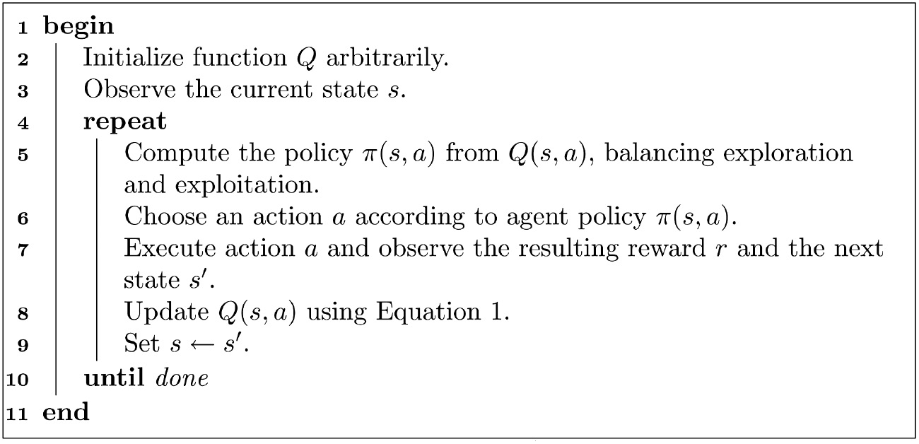
The parameter α is called the learning rate and controls the speed of learning. The variables r and s′ refer to the immediate reward and the next state, respectively (both of which are observed after executing action a at state s). Algorithm 1 illustrates how the Q-learning update equation is typically used in combination with an exploration strategy that generates a policy from the Q-values.
The agent needs to choose the next action considering that its current Q-values may still be erroneous. The belief of an action to be inferior may be based on a crude estimate, and there may be a chance that updating that estimate reveals the action’s superiority. Therefore, the function Qt in itself does not dictate which action an agent should choose in a given state (step 5 in Algorithm 1). The policy π(s, a) of an agent is a function that specifies the probability of choosing action a at state s. A greedy policy that only selects the action with the highest estimated expected value can result in an arbitrarily bad policy, because if the optimal action initially has a low value of Q, it might never be explored. [A greedy policy can be formally defined as πt(s, a)=1 iff a=argmaxa′Qt(s, a') and πt(s, a)=0 otherwise.] To avoid such premature convergence on suboptimal actions, several definitions of π have been proposed that ensure all actions (including actions that may appear suboptimal) are selected with non-zero probability [9]. These definitions of ππ are often called exploration strategies [37]. The two most common exploration strategies are ϵ-greedy exploration and Boltzmann exploration. The ϵ-greedy exploration simply chooses a random action with probability ϵ, and otherwise (with probability 1−ϵ) chooses the action with the highest Q-value greedily. In this paper, we focus on Q-learning with ϵ-greedy exploration.
Q-learning Algorithm.
 |
2.2 The Problem: Analyzing Learning Dynamics in Multi-agent Context
Analyzing the learning dynamics in a MAS is a non-trivial task, due to the large number of system parameters (each agent maintains a set of local parameters controlling its behavior), the concurrency by which these parameters change (agents acting independently), and the delay in the effect/consequence of parameter changes (because of communication delay between agents and the time it takes for learning algorithms to adapt). For instance, the Q-learning algorithm, which we briefly explained in the previous section, was analyzed more recently and only for stateless domains in a multi-agent context [20, 23, 43]. Although theoretical analysis can provide strong guarantees, it is prohibitively complex to pursue except for simple domains and simple algorithms (theoretical analysis is usually limited to systems with few agents and simple algorithms [27, 41]). Researchers usually relied on experimental analysis in large-scale systems and inspected the evolution of some global performance metrics as an approximation to the underlying learning dynamics. For example, if the system performance improved and stabilized over time, then it was assumed that learning converged. However, this can be misleading, as was shown before [1]. This section expands the motivating questions that were mentioned in Section 1. We group the questions under two main classes: parameter analysis and strategy analysis.
In Section 3, we propose methodologies that attempt to answer these questions.
Parameter analysis
A practical question that faces researchers when designing a multi-agent learning experiment is to which values shall one set the parameters of the learning algorithm? The vast majority of the previous work that evaluated multi-agent learning used the following criteria for choosing parameter values:
The values worked reasonably well (it was not explained how such values were found) [6].
Adopting parameter values from previous work [44].
Despite the importance of the parameter values, we are not aware of any methodological procedure for choosing these values. Such methodology shall not only identify good parameter values but also identify ranges of parameter values safe to use, and determine whether there is dependence between parameters.
Strategy analysis
Identifying regions of parameter values that lead to desired performance is useful, but cannot explain how such performance is achieved and learned, or if there is any common pattern in agent dynamics. It may be useful to know to which policy agents stabilize (if agents do stabilize). Also, what are the intermediate joint strategies that agents pass until reaching the stable joint policies?
2.3 Case Study: IPD
Prisoner’s dilemma (PD) is perhaps the most widely studied toy problem in economics, sociology, biology, and computer science [28, 29, 30, 34, 35]. Table 1 summarizes the game. Each agent has one of two choices: to cooperate (C) or to defect (D). One agent controls which row is selected, while the other player controls which column is selected. The numbers in the corresponding cell represent the payoff of the row player and the column player, respectively. For the row agent, the best action is to defect, whether the column player cooperates (payoff is 6) or defects (payoff is 1). The same argument goes for the column player. Therefore, both players, if selfish and shortsighted, will defect and only get the payoff of 1 each. This payoff is much less than the payoff of mutual cooperation (where each player gets a payoff of 5), hence the dilemma. Despite its simplicity, PD captures the trade-off between cooperation that leads to social welfare and selfishness that leads to poverty.
Prisoner’s Dilemma Game That Is Used in the Experiments.
| C | D | |
|---|---|---|
| C | 5,5 | 0,6 |
| D | 6,0 | 1,1 |
If players interact with one another more than once, then we have an IPD problem. In IPD, agents can use the history of interactions to model the opponent and respond accordingly, and therefore the domain becomes a multi-state domain, not a single-state or stateless domain. For example, if we only consider a history of size 1, then we have four possible states representing the combinations of two player actions: CC, CD, DC, and DD. Researchers in social sciences have developed several strategies that observed and took into account the history of the previously selected actions (usually just looking one time step behind). The tit-for-tat strategy [30] is one of the famous strategies that addressed this dilemma. Table 2 summarizes the strategy. For example, if at time t the opponent defected (chose action D), then the player will choose action D at time t+1. During the last few decades, the IPD game has been used extensively to study multi-agent learning. For example, the tit-for-tat strategy was reported to encourage Q-learners to cooperate (if Q-learning played against a tit-for-tat-player) [35]. However, even until recently, reaching and maintaining cooperation has been challenging for many reinforcement learning algorithms [17]. Section 5 reviews the previous analysis of Q-learning in the IPD domain.
The Tit-for-Tat Strategy as a Function of the State, Where Each State Consists of the Actions Chosen in the Previous Time Step.
| State | Next chosen action | |
|---|---|---|
| Self | Opponent | |
| C | C | C |
| C | D | D |
| D | C | C |
| D | D | D |
3 Methodology
This section presents the methodologies we propose to solve the problems outlined in Section 2.2.
3.1 Using Decision Trees to Discover Consistent Clusters of Learning Parameter Values
We present a methodology for solving the parameter analysis problem and later show how this has been useful in identifying parameter values that allow Q-learning to cooperate in IPD. The methodology consists of the following steps:
Data collection:Data are collected for large combinations of learning parameter values. A data tuple consists of the different parameter values along with the global performance metric achieved in the particular simulation run. For example, in the IPD domain, we collect the average payoff for different combinations of Q-learning parameters α, γ, and ϵ. Multiple simulation runs are executed, and the corresponding data are collected for the same parameter value combination to ensure the consistency of the results.
Data preprocessing: To improve the quality of the next step (decision tree construction), we preprocess the data as follows. First, the performance metric is converted from continuous values to discrete classes. In the case of IPD, for example, we convert the payoff to a binary value: either 1 if the average payoff is >4 or 0 otherwise. Second, if the percentage of a class is too low, we use stratified sampling. Stratified sampling is a technique that increases the percentage of rare classes through resampling. For example, in the IPD domain, the simulation episodes where agents learn to cooperate are significantly less than the instances where defection prevails. We have used stratified sampling to artificially increase the number of data instances where cooperation is maintained.
Decision tree construction: Using the preprocessed data, a decision tree is constructed using any available implementation. We have chosen decision trees because of their explanatory power. Figure 1 shows an example decision tree.
Rule interpretation: After the tree is constructed, a human expert can inspect the different branches and deduce interesting rules and regions of parameter values. For example, one of the rules we discovered in IPD is that agents using Q-learning will never learn to cooperate if the discount factor γ<0.75 and the learning rate α>0.148.

The Decision Tree That Is Learned from the Learning Parameters Data Set.
The majority of the paths lead to defection (class 0). Only 9 (out of 36) paths in the tree lead to cooperation.
While the data collection step above might be expensive (depending on the number of parameter combinations), the benefit of constructing the decision tree is getting a more complete and reliable picture regarding the space of parameter values. For example, suppose in a particular domain some parameter values α=0.1, γ=0.9, and ϵ=0.1 result in good performance. If these parameters change slightly, will the performance increase or decrease? Using decision trees, discover clusters or regions of parameter values that result in similar performances.
3.2 Using Sequence Analysis to Discover Patterns in Multi-state Learning Dynamics
We propose here the methodology for addressing the strategy analysis problem, which uses frequent sequence mining to discover such patterns. The methodology consists of the following steps.
Data collection: Dynamics data are collected for combinations of learning parameter values that belong to the same performance class. For example, in the IPD game, we analyze the dynamics for parameter combinations that lead to cooperation. A data tuple here is time series of data structure values. For example, in case of Q-learning, the main data structure is the Q-table, so each tuple consists of the values in the Q-table (for each state and action) at different times for the different agents in the system. In other words, for two agents, two actions, and four states, we have 16 time series per data tuple.
Data preprocessing: Because frequent sequence mining requires binary data, the preprocessing step converts any continuous time series to a binary time series. For example, in case of Q-learning, the Q-values of every pair of actions for a given agent and a given state are converted to a binary variable representing the strategy at this particular state (if the Q-value of cooperation is higher than defection, then the strategy is to cooperate, and vice versa).
Frequent sequence mining: Having prepared our data set, we can use any implementation of frequent sequence mining algorithms. A sequence shows a transition of agent strategies from one joint strategy to another. Frequent sequence mining discovers sequences that occur frequently in the data. We have used the TraMineR implementation [21].
Sequence interpretation: After frequent sequences are discovered, a human expert can inspect the sequences and identify interesting patterns. For example, one of the frequent sequences we have discovered in the IPD domain is that agents using Q-learning always learn the Pavlov strategy if they ever learn to cooperate.
4 Case Study: Analysis of Cooperation in IPD Game
In this section, we conduct an experimental analysis of the Q-learning dynamics in the IPD domain with multi-state setting (agents observe and remember the previous joint action). When Q-learning was studied in the context of IPD, it was reported that Q-learners playing against one another did not necessarily cooperate [35]. In fact, cooperation only appeared <50% of the time. Those results were obtained for specific parameter values, and agents stopped learning after some time (after a period of decaying exploration). Whatever strategy an agent reached at this point was followed thereafter [35]. Treating the process of tuning the learning parameters as a minor issue is a common practice in most of the previous work. Usually, only the successful values of learning parameters were reported [35, 45]. Here, we revisit the analysis of Q-learning in IPD and show that more careful investigation of the learning parameter values improves the promotion of cooperation significantly. Another common limitation of the previous studies of Q-learning in IPD was the lack of explanation and/or an in-depth discussion of the multi-state policy that agents learn. Although history states were used and Q-learning learned a policy for each state, this learned policy was usually overlooked and only the final outcome (e.g. the payoff and/or the percentage of cooperation) was reported. We study here how the learned policy changes over time and to what policy do agents converge to.
We conducted experimental analysis using simulation of the IPD domain. Agents were assumed to observe the previous joint action, resulting in a total of four states: CC, CD, DC, and DD. The Q-learning algorithm in this case would store eight action values (two actions×four states). We have investigated different combinations of the Q-learning parameters: α from 0.01 to 1 with 0.025 step, ϵ from 0.01 to 0.4 with 0.01 step, and γ from 0.1 to 1 with step 0.1. This is a total of 14,040 combinations. For each combination, five independent runs have been conducted, and the average payoff and the standard deviation are computed. In each simulation run, two Q-learning agents interact for 500,000 iterations. The total number of simulation runs we have conducted is 70,200 (five independent runs for each of the 14,040 combinations). Going through the records to find a combination of parameter values that lead to cooperation is relatively easy: look for parameter values that result in average payoff >4. However, trying to find patterns across these records that govern parameter values is not an easy task. We use the methodology outlined in Section 3.1 to discover such patterns, where the performance class is defined as 1 if the payoff is >4, and 0 otherwise.
Figure 1 shows the resulting decision tree that is learned from the collected data set (which includes cases of both cooperation and defection). Although the tree is relatively large, it significantly summarizes the data set of 70,200 records to just few nodes. Furthermore, only nine leaves end up with high payoff (class 1). In eight of the nine leaves, a clear condition for cooperation emerge: γ>0.75 (agents need to value future interactions favorably). We can also observe an inverse relationship between the α parameter and the ϵ parameter. For example, cooperation occurs when 0.035>ϵ>0.015 (low) and 0.198>α>0.148 (relatively high), or when 0.135>ϵ>0.155 (relatively high) and 0.073>α>0.023 (low). In other words, agents shall either explore more often but learn with a slower pace, or explore less often and learn faster.
Identifying the clusters of learning parameter values that lead to similar outcomes is useful but tells us little about the learning dynamics. We now apply the methodology outlined in Section 3.2 to analyze further the learning dynamics that lead to cooperation. We focus on cooperation rather than defection because cooperation is more beneficial and rare (only 9 out of the 36 leaves in the decision tree lead to cooperation). With four states, two actions, and two agents, we have a total of 16 continuous variables representing the dynamics of Q-learning. As a preprocessing step, we converted the Q-values of every pair of actions at a given time t, a given agent i, and a given state s to a binary variable representing the strategy:
With eight binary variables, there are 256 possible joint strategies. Trying to discover sequential patterns in such dynamics is challenging. In this part of our evaluation, we focused on three representative parameter settings that all lead to cooperation:
α=0.07, γ=0.7, and ϵ=0.07;
α=0.075, γ=0.8, and ϵ=0.125;
α=0.125, γ=0.8, and ϵ=0.025.
Each setting has been simulated for 10 runs (a total of 30 instances of cooperation). Interestingly, we found that agents never converged to the more famous and well-known tit-for-tat strategy. Instead, agents converged to the same symmetric strategy: CDDC-CDDC. This strategy (which we were not familiar with before conducting our analysis) is called the Pavlov strategy and is shown in Table 3.
The Pavlov Strategy Defined by the Actions Chosen in the Previous Time Step.
| Previous action | Next chosen action | |
|---|---|---|
| Self | Opponent | |
| C | C | C |
| C | D | D |
| D | C | D |
| D | D | C |
The Pavlov strategy was previously reported in the social sciences [30], and is a variant of win-stay-lose-switch strategies [30]. The strategy was shown to outperform the tit-for-tat strategy in evolutionary simulations due to two interesting properties [30]: it can correct occasional errors (more resilient to noise) and can exploit unconditional cooperators. Such properties make the Pavlov strategy well suited for Q-learning (promotes cooperation while being resilient to exploration).
We have conducted frequent sequence mining [21] on the sequence data sets, and few interesting patterns were discovered. Despite the existence of 256 possible joint strategies, only 3 joint strategies dominated the sequences: DDDD-DDDD, CDDD-CDDD, and CDDC-CDDC. The mined sequences showed that agents moved from DDDD-DDDD to CDDD-CDDD, and then moved to CDDC-CDDC and stabilized.
5 Related Work
Studying the dynamics of learning algorithms in multi-agent contexts has been an active area of research [6, 7, 12, 16, 18, 20, 25, 26, 28, 38, 43]. Analyzing the dynamics goes beyond observing the received payoff and attempts to understand the evolution of agent policies overtime. The vast majority of the previous work in analyzing the dynamics focused on studying the dynamics in stateless domains with very few exceptions [7, 18, 41]. Of the few exceptions, a complete coverage of the literature is beyond the scope of this paper; therefore, we will focus on the papers that are most related to our work.
One of the earliest analysis of Q-learning in IPD assumed agents keep record of previous interactions and used the Boltzmann exploration strategy [35]. Perhaps the most significant result was that Q-learning agents (using Boltzmann exploration) did not stabilize on cooperation and kept oscillating across different joint policies even after disabling exploration. There was no extensive analysis of different parameter values (results were reported only for parameter values that worked best). Also, there was no mention of which multi-state strategy did agents reach and how it compared to well-established strategies such as tit-for-tat or Pavlov [35]. More recent analysis of Q-learning with Boltzmann exploration used evolutionary (replicator) dynamics [25, 38]; however, the same methodology cannot be applied to Q-learning with ϵ-greedy exploration due to the discontinuous nature of the ϵ -greedy exploration.
The connection between Q-learning and well-established strategies was indirectly studied in a recent work [7]. That earlier work, unlike our work here, did not show that Q-learning in self-play evolves to Pavlov strategy. Instead, it reported the results if Q-learning was to interact with another fixed player that follows one of the well-known strategies such as TFT and Pavlov. It was also reported that if Q-learning was initialized to the Pavlov strategy, then cooperation could be sustained. Here, we show that even if Q-learning was not initialized to the Pavlov strategy and under range of parameter values, Q-learning will eventually converge to the Pavlov strategy. Q-learning with ϵ-greedy exploration was theoretically analyzed relatively recently [20, 43], long after Q-learning was first studied in a multi-agent context. However, the analysis was limited to stateless Q-learning and therefore did not comment on the multi-state policies that Q-learning reached. Recently, modified and extended versions of Q-learning were proposed to promote cooperation, such as individual Q-learning [26], the CoLF and CK heuristics [18], frequency adjusted Q-learning [23], and utility-based Q-learning [29]. The dynamics analysis focused primarily on the payoff and how it compared to the Nash equilibrium. We study in this paper the basic Q-learning with ϵ-greedy exploration; however, our methodology can be applied to study the dynamics of such extensions.
It is important to distinguish what we are proposing from the important research that falls under the term agent mining. Agent mining research focuses on integrating data mining with agent technologies to achieve reliable and distributed data mining [14], while we are proposing here the use of data mining techniques to analyze specific data generated by agents themselves: the multi-agent learning dynamics.
6 Conclusion and Future Work
We proposed in this paper methodological procedures that use data mining techniques to extract useful information from multi-agent learning dynamics. We provided a methodology for identifying safe regions of learning parameter values, and a methodology for detecting frequent transitions in multi-agent learning dynamics. We verified the potential of our approach using IPD (with multiple states). We were able to discover interesting information from the large dynamics data using the methodologies we proposed.
One of the future directions we plan to pursue is the use of frequent sequence mining to analyze the more complex domains of multi-agent learning dynamics, such as automated trading over networks. The data that result from integrating information about the network structure with the sequence data (of evolving agent strategies) is complex and challenging to analyze. Another important direction is developing novel visualization techniques that are suitable for multi-state dynamics.
Funding source: British University in Dubai
Award Identifier / Grant number: INF0009
Funding statement: Grant support: This work was supported in part by the British University in Dubai grant INF0009.
Bibliography
[1] S. Abdallah, Using graph analysis to study networks of adaptive agent, In: Proceedings of the International Joint Conference on Autonomous Agents and Multiagent Systems, pp. 517–524, 2010.Search in Google Scholar
[2] S. Abdallah and M. Kaisers, Addressing the policy-bias of Q-learning by repeating updates, In: International Conference on Autonomous Agents and Multi-Agent Systems (AAMAS), pp. 1045–1052, 2013.Search in Google Scholar
[3] S. Abdallah and M. Kaisers, Improving multi-agent learners using less-biased value estimators, In: Proceedings of the International Conference on Intelligent Agent Technology, 2015.10.1109/WI-IAT.2015.113Search in Google Scholar
[4] S. Abdallah and M. Kaisers, Addressing environment non-stationarity by repeating Q-learning updates, J. Mach. Learn. Res.17 (2016), 1–31.Search in Google Scholar
[5] S. Abdallah and V. Lesser, Multiagent reinforcement learning and self-organization in a network of agents, In: Proceedings of the International Joint Conference on Autonomous Agents and Multiagent Systems, pp. 1–8, 2007.10.1145/1329125.1329172Search in Google Scholar
[6] S. Abdallah and V. Lesser, A multiagent reinforcement learning algorithm with non-linear dynamics, J. Artif. Intell. Res.33 (2008), 521–549.10.1613/jair.2628Search in Google Scholar
[7] M. Babes, E. M. de Cote and M. L. Littman, Social reward shaping in the prisoner’s dilemma, in: Proceedings of the International Joint Conference on Autonomous Agents and Multiagent Systems (AAMAS), pp. 1389–1392, 2008.Search in Google Scholar
[8] P. M. Berry, M. Gervasio, B. Peintner and N. Yorke-Smith, PTIME: personalized assistance for calendaring, ACM Trans. Intell. Syst. Technol. (TIST) 2 (2011), 40.10.1145/1989734.1989744Search in Google Scholar
[9] O. Besbes, Y. Gur and A. Zeevi, Optimal exploration-exploitation in a multi-armed-bandit problem with non-stationary rewards, Available at SSRN 2436629 (2014).10.2139/ssrn.2436629Search in Google Scholar
[10] C. Boutilier, Sequential optimality and coordination in multiagent systems, In: Proceedings of the International Joint Conference on Artificial Intelligence, pp. 478–485, 1999.Search in Google Scholar
[11] M. Bowling, Convergence and no-regret in multiagent learning, In: Proceedings of the Annual Conference on Advances in Neural Information Processing Systems, pp. 209–216, 2005.Search in Google Scholar
[12] M. Bowling and M. Veloso, Multiagent learning using a variable learning rate, Artif. Intell.136 (2002), 215–250.10.1016/S0004-3702(02)00121-2Search in Google Scholar
[13] J. A. Boyan and M. L. Littman, Packet routing in dynamically changing networks: a reinforcement learning approach, In: Proceedings of the Annual Conference on Advances in Neural Information Processing Systems, pp. 671–678, 1994.Search in Google Scholar
[14] L. Cao, G. Weiss and P. S. Yu, A brief introduction to agent mining, Autonom. Agents Multi-agent Syst.25 (2012), 419–424 (English).10.1007/s10458-011-9191-4Search in Google Scholar
[15] Y. H. Chang and T. Ho, Mobilized ad-hoc networks: a reinforcement learning approach, In: Proceedings of the International Conference on Autonomic Computing, pp. 240–247, IEEE Computer Society, Washington, DC, USA, 2004.Search in Google Scholar
[16] C. Claus and C. Boutilier, The dynamics of reinforcement learning in cooperative multiagent systems, In: Proceedings of the National Conference on Artificial intelligence/Innovative Applications of Artificial Intelligence, pp. 746–752, 1998.Search in Google Scholar
[17] J. W. Crandall, Towards minimizing disappointment in repeated games, J. Artif. Intell. Res.49 (2014), 111–142.10.1613/jair.4202Search in Google Scholar
[18] J. E. M. de Cote, A. Lazaric and M. Restelli, Learning to cooperate in multi-agent social dilemmas, In: International Joint Conference on Autonomous Agents and Multiagent Systems (AAMAS), pp. 783–785, 2006.10.1145/1160633.1160770Search in Google Scholar
[19] D. Easley, M. López de Prado and M. O’Hara, The microstructure of the “Flash Crash”: flow toxicity, liquidity crashes and the probability of informed trading, J. Portf. Manage.37 (2011), 118–128.10.3905/jpm.2011.37.2.118Search in Google Scholar
[20] R. G. Eduardo and R. Kowalczyk, Dynamic analysis of multiagent Q-learning with ϵ-greedy exploration, In: Proceedings of the 26th Annual International Conference on Machine Learning, (ICML), pp. 369–376, ACM, New York, NY, 2009.Search in Google Scholar
[21] A. Gabadinho, G. Ritschard, N. S Müller and Matthias Studer, Analyzing and visualizing state sequences in R with TraMineR, J. Stat. Softw.40 (2011), 1–37.10.18637/jss.v040.i04Search in Google Scholar
[22] M. Ghavamzadeh, S. Mahadevan and R. Makar, Hierarchical multi-agent reinforcement learning, Autonom. Agents Multi-Agent Syst.13 (2006), 197–229.10.1007/s10458-006-7035-4Search in Google Scholar
[23] M. Kaisers and K. Tuyls, Frequency adjusted multi-agent Q-learning, In: Proceedings of the International Conference on Autonomous Agents and Multiagent Systems: volume 1, AAMAS’10, pp. 309–316, 2010.Search in Google Scholar
[24] J. R. Kok and N. Vlassis, Collaborative multiagent reinforcement learning by payoff propagation, J. Mach. Learn. Res.7 (2006), 1789–1828.Search in Google Scholar
[25] A. Lazaric, J. E. M. de Cote, F. Dercole and M. Restelli, Bifurcation analysis of reinforcement learning agents in the Selten’s horse game, In: Adaptive Agents and Multi-Agents Systems Workshop, pp. 129–144, 2007.10.1007/978-3-540-77949-0_10Search in Google Scholar
[26] D. S. Leslie and E. J. Collins, Individual Q-learning in normal form games, SIAM J. Control Optim.44 (2005), 495–514.10.1137/S0363012903437976Search in Google Scholar
[27] H. Li, Multi-agent Q-learning of channel selection in multi-user cognitive radio systems: a two by two case, In: Proceedings of the International Conference on Systems, Man and Cybernetics, pp. 1893–1898, Piscataway, NJ, 2009.10.1109/ICSMC.2009.5346172Search in Google Scholar
[28] K. Moriyama, Utility based Q-learning to facilitate cooperation in Prisoner’s Dilemma games, Web Intell. Agent Syst.7 (2009), 233–242.10.3233/WIA-2009-0165Search in Google Scholar
[29] K. Moriyama, S. Kurihara and M. Numao, Evolving subjective utilities: Prisoner’s Dilemma game examples, In: Proceedings of the International Conference on Autonomous Agents and Multiagent Systems, (AAMAS), pp. 233–240, Richland, SC, 2011.Search in Google Scholar
[30] M. Nowak and K. Sigmund, A strategy of win-stay, lose-shift that outperforms tit-for-tat in the Prisoner’s Dilemma game, Nature364 (1993), 56–58.10.1038/364056a0Search in Google Scholar
[31] L. Panait and S. Luke, Cooperative multi-agent learning: the state of the art, Autonom. Agents Multi-agent Syst.11 (2005), 387–434.10.1007/s10458-005-2631-2Search in Google Scholar
[32] S. Patterson, Dark Pools: The Rise of the Machine Traders and the Rigging of the US Stock Market, Crown Business, New York, NY, 2012.Search in Google Scholar
[33] L. Peshkin and V. Savova, Reinforcement learning for adaptive routing, In: Proceedings of the International Joint Conference on Neural Networks, pp. 1825–1830, 2002.Search in Google Scholar
[34] A. Rogers, R. K. Dash, S. D. Ramchurn, P. Vytelingum and N. R. Jennings, Coordinating team players within a noisy Iterated Prisoner’s Dilemma tournament, Theor. Comput. Sci.377 (2007), 243–259.10.1016/j.tcs.2007.03.015Search in Google Scholar
[35] T. W. Sandholm and R. H. Crites, Multiagent reinforcement learning in the Iterated Prisoner’s Dilemma, Biosystems37 (1996), 147–166.10.1016/0303-2647(95)01551-5Search in Google Scholar
[36] S. Singh, M. Kearns and Y. Mansour, Nash convergence of gradient dynamics in general-sum games, In: Proceedings of the Conference on Uncertainty in Artificial Intelligence, pp. 541–548, 2000.Search in Google Scholar
[37] R. Sutton and A. Barto, Reinforcement Learning: An Introduction, MIT Press, Cambridge, MA, 1999.Search in Google Scholar
[38] K. Tuyls, P. J. Hoen and B. Vanschoenwinkel, An evolutionary dynamical analysis of multi-agent learning in iterated games, Autonom. Agents Multi-agent Syst.12 (2006), 115–153.10.1007/s10458-005-3783-9Search in Google Scholar
[39] K. Tuyls and G. Weiss, Multiagent learning: basics, challenges, and prospects, AI Mag.33 (2012), 41.10.1609/aimag.v33i3.2426Search in Google Scholar
[40] K. G. Vamvoudakis, F. L. Lewis and G. R. Hudas, Multi-agent differential graphical games: online adaptive learning solution for synchronization with optimality, Automatica48 (2012), 1598–1611.10.1016/j.automatica.2012.05.074Search in Google Scholar
[41] P. Vrancx, K. Tuyls and R. Westra, Switching dynamics of multi-agent learning, In: Proceedings of the 7th International Joint Conference on Autonomous Agents and Multiagent Systems, pp. 307–313, International Foundation for Autonomous Agents and Multiagent Systems, Richland, SC, 2008.Search in Google Scholar
[42] C. J. C. H. Watkins and P. Dayan, Q-learning, Mach. Learn.8 (1992), 279–292.10.1007/BF00992698Search in Google Scholar
[43] M. Wunder, M. L. Littman and M. Babes, Classes of multiagent Q-learning dynamics with ϵ-greedy exploration, In: Proceedings of the International Conference on Machine Learning (ICML), pp. 1167–1174, 2010.Search in Google Scholar
[44] C. Zhang and V. Lesser, Multi-agent learning with policy prediction, In: Proceedings of the AAAI Conference on Artificial Intelligence, pp. 927–934, 2010.10.1609/aaai.v24i1.7639Search in Google Scholar
[45] C. Zhang and V. Lesser, Coordinated multi-agent reinforcement learning in networked distributed POMDPs, In: Proceedings of the AAAI Conference on Artificial Intelligence (AAAI), pp. 764–770, 2011.10.1609/aaai.v25i1.7886Search in Google Scholar
[46] M. Zinkevich, Online convex programming and generalized infinitesimal gradient ascent, In: Proceedings of the International Conference on Machine Learning, pp. 928–936, 2003.Search in Google Scholar
©2017 Walter de Gruyter GmbH, Berlin/Boston
This article is distributed under the terms of the Creative Commons Attribution Non-Commercial License, which permits unrestricted non-commercial use, distribution, and reproduction in any medium, provided the original work is properly cited.
Articles in the same Issue
- Frontmatter
- Extreme Learning Machine-Based Traffic Incidents Detection with Domain Adaptation Transfer Learning
- Mining Dynamics: Using Data Mining Techniques to Analyze Multi-agent Learning
- Automatical Knowledge Representation of Logical Relations by Dynamical Neural Network
- A Comparison of Three Soft Computing Techniques, Bayesian Regression, Support Vector Regression, and Wavelet Regression, for Monthly Rainfall Forecast
- Single Machine Scheduling Based on EDD-SDST-ACO Heuristic Algorithm
- Exponential Genetic Algorithm-Based Stable and Load-Aware QoS Routing Protocol for MANET
- Disruption Management for Predictable New Job Arrivals in Cloud Manufacturing
- Adaptive Fuzzy High-Order Super-Twisting Sliding Mode Controller for Uncertain Robotic Manipulator
- Intelligent Tutoring Systems
- A Novel Global ABC Algorithm with Self-Perturbing