Inertia-Based Ear Biometrics: A Novel Approach
-
M.A. Jayaram
 ,
G.K. Prashanth
,
G.K. Prashanth
 and
Sachin C. Patil
and
Sachin C. Patil

Abstract
The human ear has been deemed to be a source of data for person identification in recent years. Ear biometrics has distinct advantages, such as visibility from a distance and ease with which images could be captured. This paper elaborates on a novel approach to ear biometrics. We propose moment of inertia-based biometric for the ears in any random orientation. The features concerned are the moment of inertia about the major and minor axes, corresponding radii of gyration, and the planar surface area of the ear. The databases of the said features were collected through ear images of 600 subjects. Principal component analysis of the features demonstrated that the radius of gyration with respect to the major axis, moment of inertia about the minor axis, and radius of gyration about the minor axis are significant attributes contributing to major variability. The person identification system developed showed recognition rates of 99% with just three attributes, when compared with the 96% recognition rate when all five attributes were considered. The evaluation of the system was done on several metrics. All metrics were found to be insignificant in their magnitude, which is suggestive of robustness and excellent authentication performance.
1 Introduction
Copious literature has brought to the fore the proven advantages of ear biometrics when compared with others. To mention a few, the ears have a rich and stable structure that changes little with age, their configuration remains intact with changes in facial expression, and they are firmly attached in the middle of the side of the head so that the immediate background is predictable. Ear image collection does not have an associated hygiene issue, as may be the case with contact biometrics, and is unlikely to cause anxiety as may happen with iris and retina measurements [28].
The ear is large compared with the iris, retina, and fingerprint. Therefore, it is more easily captured at a distance. As a comparison, face recognition usually requires the face to be captured against a controlled background. Facial biometrics fail due to the changes in features caused by expressions, cosmetics, hair styles, growth of facial hair, as well as the difficulty of reliably extracting them in an unconstrained environment exhibiting imaging problems such as lighting and shadowing [8]. In the same token, though the features of the iris remain relatively consistent over time and are easy to extract, the acquisition of the image at the necessary resolution from a distance is difficult.
The ear as a biometric is no longer in its infancy and has shown encouraging progress thus far, and is improving. This is particularly seen with the interest created by the recent research into its three-dimensional (3D) potential [36]. The ear enjoys forensics support, and its structure appears individualistic. The ears, with their deep 3D structure, are simply inimitable. These aspects ensure that the ear will occupy a special place in situations requiring a high degree of protection against impersonation.
Two approaches are currently followed by researchers in the area of ear recognition. The first one is the statistical approach such as principal component analysis (PCA) [10] that results in obtaining a set of eigenvectors. An image is represented using a weighted combination of eigenvectors. The weights are obtained by projecting the image into eigenvector components using an inner product operation. The identification of the image is done by locating the images in the database whose weights are the closest to the weights of the test image. The second category is based on the local features of the ear, such as the geometry features composed of distance and curve relationship [19], or the force field feature composed of potential wells and potential channels [7]. This paper proposes a novel methodology to recognize 2D human ear by using the fundamental properties of a planar surface: the area, the moment of inertia (MI) about the major and minor axes, and the radius of gyration about the major and minor axes. The features used in this approach are invariant because the height, width, and outer shape of the ear will remain the same over the years. Thus, there will be no vital changes that will happen in the extracted features of the ear. Further, the MI and radius of gyration are the two physical properties of any planar surface that signifies the shape and the resistance offered by the planar surface against rotation about an axis.
The rest of the paper is organized in the following manner. Section 2 elaborates the related works. The proposed methodology is presented in Section 3. The process adopted for data acquisition is described in Section 4. A detailed explanation of features and feature extraction is done in Section 5. PCA and consequent identification of significant features through PCA is demonstrated in Section 6. Elaboration on the person identification system and recognition of persons using significant ear biometric features identified by PCA is presented in Section 7. Conclusions are drawn in Section 8.
2 Related Work
Several studies on the uniqueness of ear biometrics have been reported. An extensive examination of 10,000 ears in terms of distance between predicated points has been cited [21]. However, the research finding was limited due to inadequate estimation accuracy. Researchers have also characterized the ears using the Voroni diagram [5, 6]. The work seemed to be conceptual and sans experimental results.
A method based on localized ear shape features using force field transformation has been reported by Hurley et al. [19]. In this work, a database of 63 subjects was used to demonstrate the concept. In this study, PCA was used to characterize the ear on the basis of eigenvalues connoted as eigen-ear.
Mu et al. [27] have attempted on characterizing ear shape using the gradient of ear image. Databases of 460 ears were used for features extraction. The geometric features that describe the shape information were the distance between the two reference points. In this study, N points were sampled at every 180/N degree. The (N−1) distance between such N points were taken as the feature set for an ear. The Euclidian distance between such shape features were used to compare the matching distance for ear identification.
Geometrical features extraction from ear images is the most widely accepted procedure. This approach is motivated by actual procedures used in police and forensic evidences search applications. Geometric features such as size, width, height, and earlobe topology have been considered [11–14]. Contours within the images have been captured to provide important information allowing ear description, representation, and calculation of parameters for recognition [30].
Yuan and Tian [37] have presented an ear contour detection algorithm based on a local approach. In their work, edge tracking was applied to three regions in which contours were extracted in order to obtain a clear, connected, and non-distributed contour that might further be used in the recognition step. PCA has been used for comparing ear and face properties [10, 35] in order to identify humans in various conditions. In this case, the researches used a set of eigen-faces and eigen-ears.
Lu et al. [26] used so-called active shape modules to model the shape and local appearances of the ear using a statistical approach. These shape modules were used in classification. They reported to have achieved a recognition rate of 95.1% with this kind of biometrics.
Hurley et al. [19, 20] used the energy features of 2D images. They proposed force field transformation in order to find energy line channels and wells in the ear. The researchers treated each pixel in the image as the force field source directed at all the other pixels. Force field transformation was performed to localize a small number of energy maxima. Continuing further, the authors computed the statistical parameters describing distance and angles between the detected energy maxima. In this research, a 90% recognition rate was reported.
Polin et al. [32] presented 2D human ear recognition using geometric features; in their study, they considered the ear height line (the longest) that can be drawn with both its end points on the edge of the ear, and the length was measured as Euclidean distance. The reference lines that are parallel to the width of the image and that divides the image in N+1 parts (they have also made the angle to vary from 0 to π, measuring from the highest axis to several radial lines) of 120 ear images were used for a classification task based on these geometric features.
Ear anatomy features such as Helix Rim, Lobule, Triangular Fossa, Concha, and Tragus were used for person identification. The system proposed runs in two modes, i.e. registration and identification modes. In the registration mode, the features were measured and the resulting vectors of features were compared with the template features in the database during the identification mode [22].
The curve of the outer edge of the ear is considered as a biometric, and it was assumed to be parabolic in a previous study [34]. The researchers developed a quadratic equation of the form a+bx+cx2, using seven points on the edge of the ear identified by the radial line from the center of the height axis. Making use of this equation, they calculated the area and used it as a biometric. In this work, a detection accuracy rate of 96.8% was reported.
Texture-based ear recognition has been gaining momentum in recent years. It was found that texture-based biometric descriptors are robust against signal degradation, and encoding artifact texture descriptors along with the depth information over the surface ear has been used for identification [31].
An autoregressive (AR) [24] modeling technique has been explored for identification of persons using ear biometrics. For this purpose, a time series was obtained from the contour coordinates of the ears. AR was fitted to the time series, and AR coefficients were considered as feature vectors. Recognition was done by a classifier that is based on Euclidean distance. Further, the vector of a test sample was matched with training samples within itself (intra-class) and with respect to others. The model was found to be invariant to posture, rotation, and illumination. A recognition rate of up to 99% was reported.
A person unique recognition system using a Universality, Distinctiveness, Permanence, and Measurability process to characterize the human ear, and hence to find uniqueness recognition of a person, has been attempted [25]. The researchers developed a scoring function for each ear. The scoring function was individual scores such as the Helix score, Lobule, Concha score, etc., during each feature matching. A tolerance of ±15% was kept. The system output was tested, and the reliability was found to be around 80%.
Alay-ay et al. [2] recently reported on an ear shape-based human detection system named as Oto-ID. This system was developed to provide security over prolonged user interaction. It implements ear recognition for login and uses shape-based human detection to continuously detect human presence. PCA and feature extraction are the approaches implemented in this research. Detection accuracy rates of 87.5% were found during pose variation, and have shown 100% if the distance between the ear and the camera is in the range of 40–50 cm.
PCA is a procedure considered with elucidating the covariance structure of a set of variables. In essence, it allows identifying the principal direction in which the data vary [29]. In computational terms, the principal components are found by calculating eigenvectors and eigenvalues of the data covariance matrix. The process is equivalent to finding the new axis system in which the covariance matrix is diagonal. The eigenvector with the largest eigenvalue is the direction of greatest variation, the one with the second largest eigenvalue in the orthogonal direction with the next highest variation, and so on.
PCA has two objectives:
Reducing the number of variables comprising the dataset, while retaining the variability in the data.
Identifying the hidden patterns in the data and classifying them according to how much of information stored in the data, they account for.
In this work, PCA is used to extract the unique features of the query ear, which distinguishes it from other ears [4]. Discrete cosine transformation is used to reduce the size of the dataset so that the most relevant intensity of the query image is contented in the few lower-order frequency components. In another work [1], 2D PCA has been used for face recognition on the three well-known face image databases (ORL, AR, and YALE); in all three applications, the recognition rate of PCA was found to be superior.
In yet another work [38], a robust PCA was used for modeling the biometric features of the ear; in this work, wavelet-based analysis was rendered to discriminate the boundary structures of an ear. The hybrid method involving PCA and wavelet analysis has shown to be a promising approach to ear biometrics.
3 The Proposed Method
This paper presents a thoroughly novel approach for personal identification using 2D ear images. The approach is based on the planar surface characteristic, the MI, and the related functions. In this method, the ear images were considered to be planar surfaces of irregular shape. Fundamentally, MI is the property of a planar surface that originates whenever one has to compute the moment of distributed load that varies linearly from the moment axis. A typical example of this kind of loading occurs due to the pressure of a liquid or air acting on the surface of a plate [18]. By definition, the MIs of the differential planar area, da, about two axes are respectively
For the entire area, the MIs are determined by integration, if the area is continuous [18]
If the planar surface is made up of discrete elementary areas [18], then MI is computed by summation:
where i=1, 2, …, n, are discrete elementary areas. A geometrical representation of the concept of MI is shown in Figure 1.
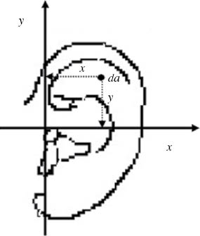
Geometrical Representation of the MI of a Differential about Two Axes.
MI also signifies the disposition or arrangement of the area with respect to a reference axis. MI is also viewed as a physical measure that signifies the shape of a planar surface, and it is proved that by configuring the shape of a planar surface and hence by altering the MI, the resistance of the planar surface against rotation with respect to a particular axis could be modulated or altered [33]. Therefore, in this work, the MIs of the ear surface with respect to two axes, i.e. the major axis and the minor axis, are considered to be the best biometric attributes that could capture the shape of the irregular surface of the ear in a scientific way. As far as the tendency of rotation of an ear is concerned, it is presumed that an ear can rotate with respect to the major axis and can be folded about the minor axis.
4 Data Acquisition
The ear images used in this work were acquired from students of the Siddaganga group of institutes. The subjects involved were mostly students and faculty numbering around 600. In each acquisition session, the subject sat approximately 1 m away, with the side of the face in front of the camera in an outdoor environment without flash. The images were obtained simultaneously. Care was taken to provide the same illumination conditions for all the captures. All images were enrolled in the gallery of a database. A cross section of the sample database is presented in Figure 2.

A Gallery Sample Database.
The images so obtained were resized in such a way that only the ear portion covers the entire frame having a pixel matrix. The color images were converted into gray-scale images followed by the uniform distribution of brightness through a histogram equalization technique. The delineation of the outer edge of each ear was obtained using a canny edge detection algorithm. The resulting edge was inverted to get a clear boundary shape of the ear. The conceptual presentation of the process involved is shown in Figure 3. One typical edge of an ear boundary is shown in Figure 4.

Steps Involved in Ear Edge Extraction.

Outer Edge of Ear (Typical).
5 Feature Extraction
To start with, the major axis and minor axis were identified. The major axis is the one that has the longest distance between two points on the edge of the ear; the distance here is the maximum among the point-to-point Euclidean distances. The minor axis is drawn in such way that it passes through the tragus and is orthogonal to the major axis. Therefore, with different orientations of the ears, the orientation of the major axis also changes. Being perpendicular to the major axis, the orientation of the minor axis is fixed.
The surface area of the ear is the projected area of the curved surface on a vertical plane. This area is assumed to be formed out of segments. The area of an ear to the right side of the major axis is considered to be made out of six segments. Each of the segments thus subtends 30° with respect to the point of the intersection of the major axis and minor axis. The extreme edge of a sector is assumed to be a circular arc, thus converting each segment into a sector of a circle of varying area. One such typical segment is shown in Figure 5, and a measurement involved over such segment is presented in Figure 6.

Features of the Ear.

Centroid Location of the Circular Sector Area.
The measurements are as follows:
θ: inclination of the central radial axis of the segment with respect to minor axis (in degrees);
r: the length of the radial axis (in mm).
The conversion of the number of pixels into a linear dimension (in mm) was based on the resolution of the camera expressed in PPI (pixels per inch). In this work, a 16-megapixel camera at 300 PPI was used. The computation of linear distance is straightforward: mm=(number of pixels*25.4)/PPI (1 in.=25.4 mm). With these measurements, the following parameters are computed.
MI with respect to the minor axis Imin
where ai is the area of a the ith segment and yi is the perpendicular distance of the centroid of the ith segment with respect to the minor axis:
Here, C is the centroidal distance of the segment with respect to the intersection point of the axes, which is given by [38]
Similarly, the MI with respect to the major axis Imax, xi, is the perpendicular distance of the centroid of the ith segment with respect to the major axis.
From the computed values of MI and area of the ear surface, the radii of gyration with respect to the minor axis (RGx) and the major axis (RGy) were computed. The formulae for radii of gyration are given by [15]
where A is the sum of the areas of six segments:
A section of the right ear feature database is presented in Table 1.
Calibration of the area
A Sample Database (Right Ear).
| A (mm2) | Imin (mm4) | Imax (mm4) | RGx (mm) | RGy (mm) | Major axis (mm) | Minor axis (mm) |
|---|---|---|---|---|---|---|
| 1054.09 | 13,548.79 | 33,529.17 | 2.46 | 5.68 | 50.62 | 29.47 |
| 1477.39 | 18,653.79 | 35,448.46 | 1.85 | 4.76 | 55.45 | 19.90 |
| 1815.42 | 20,458.75 | 44,501.02 | 4.37 | 5.70 | 65.74 | 29.27 |
| 1641.17 | 21,354.79 | 38,746.51 | 2.15 | 4.86 | 53.06 | 26.00 |
| 1759.08 | 18,546.79 | 40,263.80 | 3.24 | 5.61 | 64.47 | 30.54 |
| 1947.47 | 14,568.75 | 45,021.31 | 1.26 | 4.16 | 66.59 | 26.05 |
| 1856.08 | 22,903.51 | 44,550.11 | 1.08 | 2.15 | 65.25 | 25.52 |
| 1630.32 | 61,208.56 | 38,520.81 | 2.07 | 5.27 | 61.17 | 22.96 |
| 1909.18 | 28,157.12 | 44,980.40 | 1.81 | 5.80 | 65.86 | 24.96 |
| 1212.87 | 16,271.48 | 35,089.56 | 1.61 | 8.73 | 49.63 | 16.22 |
| 1054.09 | 13,637.79 | 33,619.17 | 2.66 | 5.86 | 52.22 | 29.52 |
| 1477.38 | 18,766.75 | 35,529.46 | 1.41 | 4.75 | 55.84 | 19.93 |
| 1815.42 | 20,314.31 | 44,056.13 | 4.24 | 5.51 | 65.17 | 29.33 |
| 1641.17 | 21,210.35 | 38,301.63 | 2.02 | 4.67 | 54.65 | 25.03 |
| 1759.08 | 18,402.35 | 39,818.91 | 3.11 | 5.42 | 64.30 | 29.50 |
| 1947.47 | 14,424.31 | 44,576.42 | 1.14 | 3.97 | 66.80 | 26.12 |
| 1856.08 | 22,759.07 | 44,105.22 | 0.95 | 1.96 | 65.77 | 24.90 |
| 1630.32 | 61,208.56 | 38,520.81 | 2.07 | 5.27 | 61.10 | 23.05 |
| 1909.18 | 28,157.12 | 44,980.40 | 1.81 | 5.80 | 65.05 | 24.96 |
| 1212.87 | 16,271.48 | 35,089.56 | 1.61 | 8.73 | 18.93 | 17.21 |
The computation of the surface area of the ear was based on the assumption that the boundary of each segment is circular. This assumption results in a cumulative error across all the six segments because the edge of the ear is not made of perfect circular arcs. To account for this error, the actual area of each and every ear in the database is measured by using a digital planimeter. A digital planimeter is used for the measurement of area bounded by irregular shapes. Planimeters have found their wide applications for many years. The instrument is shown in Figure 7A. To measure the area subtended by a closed irregular curve, the object is placed below the probe of a rotating arm that has a lens and cross hairs for accurate alignment of the curved boundary with respect to the moving arm. This instrument was designed on the basis of a quantization process. A planimeter exhibits excellent accuracy typically at 0.2% [3]. The accurate surface areas of all the ear samples were measured by using the digital planimeter manually. The experimental setup is shown in Figure 7B.

Calibration of Computed Area. (A) Digital Planimeter. (B) Area Measurements Using the Digital Planimeter.
With computed area (on the image) and actual area (using the planimeter), a non-linear regression analysis was carried out using Excel. The regression equation of the curve was found to be
where Ac is calibrated area, a is the computed area, and 1837.9 and 11,910 are regression constants.
Figure 8 shows the regression curve along with the scattering of the points. It can be seen from the curve that there is only a minor magnitude of scattering. The analysis of error incurred in computation of area was also done. The root mean square error value was found to be as low as 125. Added to this, the average error between the computed area through image measurements and the actual area through the planimeter of all the ears was also found to be 4.66%. These two measures are suggestive of the fact that the computational error involved in the planar surface area is marginal. The computed area of the ear is the input for the calibration equation to obtain the exact area of the ear as the output, thus obtaining the exact area by the system.

Curve of Best Fit.
As it is not prudent to present the complete data repository of the ears, a descriptive statistics analysis of attribute data was done. Table 2 presents the descriptive statistics of the entire data of the right ear. Descriptive statistics gives a summary of the collected data in a clear and understandable way. The central tendency of the data is depicted by mean and median of all the nine features of all the ears. The range measures the dispersion of the data. The skewness, measures the deviation of the distribution of the data the value indicates that the distribution of all the parameters is asymmetric. Kurtosis, which is an indicator of the peakedness of the distribution, is clearly different from zero, which indicates that the distribution is more peaked than normal. Standard deviation and variance indicate the scatterness of attribute values with respect to their average. There is an appreciable value of standard deviation and variance for all the attribute values which intern indicates that there is a variability in these attributes.
Descriptive Statistics of Ear Features for the Entire Database.
| S. no | M1 (mm) | M2 (mm) | A1 (mm2) | A2 (mm2) | A (mm2) | Imax (mm4) | Imin (mm4) | RGx (mm) | RGy (mm) | |
|---|---|---|---|---|---|---|---|---|---|---|
| 1 | Mean | 62.315676 | 23.11342 | 1029.09 | 928.7715 | 1920.519 | 63,249.8548 | 37,828.8147 | 7.189329 | 3.53472 |
| 2 | Median | 63.206 | 23.2102 | 928.1938 | 840.9659 | 1737.422 | 42,775.6391 | 23,230.3368 | 6.618619 | 3.205432 |
| 3 | Standard deviation | 6.8614911 | 4.048732 | 366.7951 | 366.0958 | 694.3276 | 91,346.1497 | 57,085.9967 | 2.520325 | 1.693496 |
| 4 | Variance | 47.080061 | 16.39223 | 134538.7 | 13,4026.1 | 482,090.8 | 8,344,119,073.00 | 3,258,811,020.00 | 6.35204 | 2.867927 |
| 5 | Kurtosis | 3.0328662 | −0.82716 | 0.00591 | 0.011218 | 0.10165 | 42.0363847 | 10.8897931 | −0.26037 | 2.277937 |
| 6 | Skewness | −0.9525944 | −0.13208 | 0.739706 | 0.734531 | 0.830819 | 6.19088895 | 3.47763469 | 0.588988 | 1.151528 |
| 7 | Min | 18.934 | 13.4247 | 331.1722 | 229.2122 | 553.5184 | 2884.27825 | 1593.23797 | 1.862836 | 0.8134 |
| 8 | Max | 73.9466 | 31.9485 | 2268.063 | 2166.103 | 4097.718 | 802,410.363 | 310,819.142 | 14.84563 | 11.9742 |
| 9 | Range | 55.0126 | 18.5238 | 1936.891 | 1936.891 | 3544.2 | 799,526.085 | 309,225.904 | 12.9828 | 11.1608 |
M1, major axis; M2, minor axis; A1, area above the minor axis; A2, area below the minor axis; A, total area.
6 PCA of the Feature Set
The purpose of conducting PCA on the entire data set in our work is to reduce the number of attributes and retain only significant attributes, to hasten the recognition rate. PCA was done using five features, namely the planar surface area of the ear, MI with respect to the major axis, MI with respect to the minor axis, radius of gyration about the minor axis, and radius of gyration about the major axis. Table 3 shows the covariance matrix of these features. It is seen from Table 3 that there exists a positive correlation among the features. PCA was carried out by diagonalization of the covariance matrix. Table 4 summarizes PCA results in terms of eigenvalues and eigenvectors. The amount of variance spanned by each principal component depends on the relative magnitude of its eigenvalues with respect to total sum of eigenvalues. There are several criteria to identify the number of principal components to be retained in order to understand the underlying structure of feature data. In this work, a bar chart of eigenvalues (Figure 9) was used. This bar chart shows a change in slope after the third eigenvalue, which suggests that it is enough to use only three principal components having a sum of eigenvalues at 3.87 explaining 77.4% of the variance contained in the original feature set. PC1 explains 42% of the variance and is contributed by the radius of gyration about the major axis; this is followed by 32% of the variance contributed by the MI with respect to the minor axis; and PC3 explains 26% of the variance contributed by the radius of gyration with respect to the minor axis, thus proving the significance of these among the five features of ear recognition. Further, the significance of feature reduction as elicited by PCA comes from the fact that the system developed is needed to cater to a sizable number of pupils (numbering around 10,000) in Siddaganga Education Society.

Bar Chart of Eigenvalues of PCA.
Covariance Matrix of Features.
| A | Imax | RGy | Imin | RGx | |
|---|---|---|---|---|---|
| A | 1.0000 | ||||
| Imax | 0.4514 | 1.0000 | |||
| RGy | −0.0390 | 0.2975 | 1.0000 | ||
| Imin | 0.1237 | 0.0029 | 0.0164 | 1.0000 | |
| RGx | 0.0207 | 0.0792 | 0.2819 | 0.1455 | 1.0000 |
Eigenvalue and Eigenvector of Principal Components.
| PC1 | PC2 | PC3 | |
|---|---|---|---|
| RGy | −0.4454 | −0.5021 | 0.3542 |
| Imin | −0.1993 | −0.1075 | −0.8634 |
| RGx | −0.3528 | −0.5845 | −0.1853 |
| Eigenvalues | 1.6081 | 1.2114 | 1.0477 |
| % Variability | 42 | 32 | 26 |
7 Person Identification System
The identification experiments were performed on the existing database of collected images. In the first phase, all the five attributes were considered, for which the system showed a recognition rate of 96%. In the second phase, only three features as elicited by PCA were considered. In this case, the recognition rate was 99% and also the process became fast owing to a substantial reduction in the computation of biometric parameters. In both phases, the matching of the features was performed by computing the Euclidian distance. For this purpose, the threshold value of differential Euclidian distances between the test image and the template images were found empirically, and it was found to be in the range of 1*10–3 to 1*10–6. The procedure of matching and consequent identification is depicted by a flowchart as shown in Figure 10. The details of the recognition rate are shown in Table 5. A snapshot of the identification system with three features is shown in Figure 11. The process time was measured for both cases. It was found that, with five biometric features, the average increase in the CPU time was around 12.2%. Table 6 shows the average CPU times.
Recognition Accuracy.
| With five features | With three features | ||||
|---|---|---|---|---|---|
| No. of test images | No. of correctly identified images | Percentage | No. of Test Images | No. of correctly identified images | Percentage |
| 200 | 192 | 96 | 200 | 198 | 99 |
Average Process Time (in Seconds).
| With five features | With three features |
|---|---|
| 0.98 | 0.86 |

Functioning of Ear Recognition System.

Typical Snapshot of the Identification System of Three Features.
8 Evaluation of the System
Accurate automatic personal identification is critical to a wide range of application domains such as access control e-commerce, etc. In this direction, the evaluation of identification systems becomes crucial [23].
The evaluation of a biometric system can be categorized into three main types based on (i) data quality, (ii) usability, and (iii) security [16].
Evaluation of data quality is about controlling the quality of the biometric raw data using quality information. At this stage, the poor-quality samples are removed during the enrollment phase. In our work of 655 samples, 55 samples were not considered while developing the system because of bad quality.
Usability, according to ISO 13407:1999, is defined as the extent to which a product can be used by specified users to achieve specified goals with effectiveness, efficiency, and satisfaction in a specified context of use [16]. The related metrics under this category are briefly as follows:
Fundamental performance metrics
Failure-to-enroll (FTE) rate: proportion of the user population for whom the biometric system fails to capture or extract usable information from the biometric sample.
Failure-to-acquire (FTA) rate: proportion of verification or identification attempts for which a biometric system is unable to capture a sample or locate an image or signal of sufficient quality.
False-match rate (FMR): the rate for incorrect positive matches by the matching algorithm for single-template comparison attempts.
False-non-match rate (FNMR): the rate for incorrect negative matches by the matching algorithm for single-template comparison attempts.
Verification system performance metrics
False rejection rate (FRR): proportion of authentic users that are incorrectly denied. If a verification transaction consists of a single attempt, the false reject rate would be given by
(14)False acceptation rate (FAR): proportion of impostors that are accepted by the biometric system. If a verification transaction consists of a single attempt, the false accept rate would be given by
(15)
Identification system performance metrics
Identification rate (IR): the identification rate at rate r is defined as the proportion of identification transactions by users enrolled in the system in which the user’s correct identifier is among those returned.
False-negative identification-error rate (FNIR): proportion of identification transactions by users enrolled in the system in which the user’s correct identifier is not among those returned. For an identification transaction consisting of one attempt against a database of size N, it is defined as
(16)False-positive identification-error rate (FPIR): proportion of identification transactions by users not enrolled in the system, where an identifier is returned. For an identification transaction consisting of one attempt against a database of size N, it is defined as
(17)
This is about designing a system to withstand potential threats when employed in security-critical applications. This kind of evaluation is not attempted in this work. The actual values of all the metrics discussed are presented in Table 7. All the metrics meant for evaluating the system are found to be in tune with international standards [17].
Various System Performance Measures.
| FTE | FTA | FMR | FNMR | FRR | FAR | FNIR | FPIR |
|---|---|---|---|---|---|---|---|
| 0.0 | 0.01 | 0.00 | 0.00 | 0.01 | 0.0 | 0.01 | 0.99 |
The authentication performance of the system is quantified in terms of both the FRR and FAR [17] for a foolproof system. In this context, the FRR is fixed at ≤1%, while the FAR is at 1% [17]. As far as the system is concerned, the FRR stands at 0.01% and FAR is 0%, which are indicative of its robustness in terms of authentication performance. As per the literature, an FPIR of just 0.99% is laudable because the requirement of obtaining near perfection is extremely difficult. The other metrics such as FNIR at a level of just 0.01% are highly insignificant. The rest of the metrics, i.e. FTE at 0%, FTA at just 0.01%, FMR at 0%, and FNMR at 0%, provide substantial testimony to conclude that the system developed is highly reliable and robust.
9 Conclusion
This paper presented a new set of biometric features that are based on the shape of the ear considering it as planar surface, i.e. the shape constituted just by the virtue of the outer boundary of ear and the enveloped area. The MI of the ear with respect to the major and minor axes and the related parameters, i.e. radii of gyration with respect to the major and minor axes, were the features considered. A person identification system was also developed, and the recognition system was tested considering all the features in the first phase and only the significant features enunciated by PCA in the second phase. The outcome of this research is summarized as follows:
This work involves novel biometric features based on the planar surface property that also captures the shape of the ear.
A significant reduction in computation time of features on the test image and a quick identification was achieved.
A high recognition rate of 99% was obtained when only PCA-elicited significant features were considered.
The system has also been evaluated on several functionality metrics. It was found to be in compliance with available standards and they are at desirable levels, evidencing the prudency of the system.
Bibliography
[1] H. Abdi and L. J. Williams, Principal Component Analysis Overview, vol. 2, July 2010, John Wiley and Sons, New York.10.1002/wics.101Search in Google Scholar
[2] K. M. Alay-ay, M. A. L. Meralips, D. R. Romero, R. F. Sison and B. E. V. Comendador, Oto-ID ear recognition and shape based human detection for user identification, Journal of Automation and Control Engineering3 (2015), 146–150.10.12720/joace.3.2.146-150Search in Google Scholar
[3] J. E. Allos, S. Saadallah and E. A. Hasso, A digital planimeter for industrial applications, IEEE Transaction on Industrial ElectronicsIE-31 (1984), 152–156.10.1109/TIE.1984.350060Search in Google Scholar
[4] J. Ashok and E. G. Rajan, Principal component analysis based image recognition, International Journal of Computer Science and Information Technologies1 (2010), 44–50.Search in Google Scholar
[5] M. Burge and W. Burger, Ear biometrics in machine vision, in: Proceedings of the 21st Workshop of the Australian Association for Pattern Recognition, 1997.Search in Google Scholar
[6] M. Burge and W. Burger, Ear biometrics, in: Biometrics: Personal Identification in Networked Society, A. K. Jain, R. Bolle, S. Pankanti (Eds.), pp. 273–286, 1998.10.1007/0-306-47044-6_13Search in Google Scholar
[7] M. Burge and W. Burger, Ear biometrics in computer vision. in: The 15th International Conference of Pattern Recognition, ICPR, pp. 822–826, 2000.Search in Google Scholar
[8] M. Burge and W. Burger, Ear biometrics in computer vision, in: Proc. ICPR 2000, pp. 822–826, 2002.Search in Google Scholar
[9] S. H. Cha and C. C. Tappert, Multivariate biometric matching modules technical report, Seiden Berg School of Computer Science and Information Systems, 2009.Search in Google Scholar
[10] K. Chang, K. W. Bowyer, S. Sarkar and B. Victor, Comparison and combination of ear and face images in appearance based biometrics, IEEE Transactions on Pattern Analysis and Machine Intelligence25 (2003), 1160–1165.10.1109/TPAMI.2003.1227990Search in Google Scholar
[11] M. Choras, Ear biometrics based on geometrical methods of feature extraction, in: Articulated Motion and Deformable Objects, LNCS 3179, F. J. Pearles and B. A. Draper (Eds.), pp. 51–61, Springer-Verlag, Berlin, 2004.10.1007/978-3-540-30074-8_7Search in Google Scholar
[12] M. Choras, Ear biometrics based on geometrical feature extraction, Journal ELCVIA (Computer Vision and Image Analysis)5 (2005), 84–95.10.5565/rev/elcvia.108Search in Google Scholar
[13] M. Choras, Further development in geometrical algorithms for ear biometric, in: Articulated Motion and Deformable Objects, AMDO 2006, LNCS 4069, F. J. Pearles and B. A. Draper (Eds.), pp. 58–67, Springer-Verlag, Berlin, 2006.10.1007/11789239_7Search in Google Scholar
[14] M. Choras and R. S. Choras, Geometric algorithms of ear contour shape representation and feature extraction, in: Proceedings of Intelligent System Design and Applications (ISDA), vol. II, pp. 451–456, IEEE CS Press, Jinan, China, October 2006.10.1109/ISDA.2006.253879Search in Google Scholar
[15] B. M. Das and P. C. Hassler, Statics and Mechanics of Materials, Prentice Hall, Upper Saddle River, NJ, 1988.Search in Google Scholar
[16] M. El-Abed and C. Charrier, Evaluation of biometric systems, book chapter, Intech Open Science, 2012.10.5772/52084Search in Google Scholar
[17] J. Giermanski and P. Lodge, The problem of errors, DHS, and the false positive standard, October 2007, Journal of Homeland Security, Available at: http://www.homelandsecurity.org/newjournal/articles/giermanski_dhs_false_pos.htm. Accessed 24 March, 2015.Search in Google Scholar
[18] R. C. Hibbeleer, Engineering Mechanics Dynamics, 13th ed., Prentice Hall, Upper Saddle River, NJ, June 2014.Search in Google Scholar
[19] D. J. Hurley, M. S. Nixon and J. N. Carter, Force field energy functional for image feature extraction, Image and Vision Computing20 (2002), 311–318.10.5244/C.13.60Search in Google Scholar
[20] D. J. Hurley, M. S. Nixon and J. N. Carter, Force field energy functional for ear biometrics, Computer Vision and Image Understanding98 (2005), 491–512.10.1016/j.cviu.2004.11.001Search in Google Scholar
[21] I. Iannerelli, Ear Identification, Forensic Identification Series, Paramount Publishing Company, Fremont, CA, 1989.Search in Google Scholar
[22] T. S. Indi and S. D. Raut, Person unique identification based on the ears biometric features, in: International Conference on Intelligent System and Signal Processing, 2013.10.1109/ISSP.2013.6526888Search in Google Scholar
[23] A. Jain and S. Pankanti, Biometric system: anatomy of performance, IEICE Transactions FundamentalsE00A (2001).Search in Google Scholar
[24] F. Khursheed and A. H. Mir, AR model based human identification using ear biometrics, International Journal of Signal Processing, Image and Pattern Recognition7 (2014), 347–360.10.14257/ijsip.2014.7.3.28Search in Google Scholar
[25] G. S. Kmatchi and R. Gnanajeyaraman, Ear as a raised area for hottest biometric solution using Universality, Distinctiveness, Permanence and Measurability Properties – PURS using UDPM, in: World Congress on Computing and Communication Technologies, 2014.10.1109/WCCCT.2014.57Search in Google Scholar
[26] L. Lu, X. Zhang, Y. Zhao and Y. Jia, Ear recognition based on statistical shape model, Proceedings of the International Conference on Innovative Computing, Information and Control, vol. 3, pp. 353–356, IEEE, 2006.Search in Google Scholar
[27] Z. Mu, L. Yuan, Z. Xu, D. Xi and S. Qi, Shape and structural feature based ear recognition, in: Sino Biometrics 2004, LNCS, pp. 663–670, vol. 3338, 2004.10.1007/978-3-540-30548-4_76Search in Google Scholar
[28] M. S. Nixon, I. Bouchrika, B. Arbab-Zavar and J. N. Carter, On use of biometrics in forensics: gait and ear, in: European Signal Processing Conference, 2010.Search in Google Scholar
[29] P. K. Pandey, Y. Singh and S. Tripathi, Image processing using principal component analysis, International Journal of Computer Applications15 (2011), 37–40.10.5120/1935-2582Search in Google Scholar
[30] F. A. Pellegrino, W. Vanzella and V. Torre, Edge detection revisited, in: IEEE Transactions on Systems, Man and Cybernetics, Part B34 (2004), 1500–1518.10.1109/TSMCB.2004.824147Search in Google Scholar
[31] A. Pflug, P. N. Paul and C. Busch, A comparative study on texture and surface descriptors for ear biometrics, Available at: https://www.dasec.h-da.de/wp-content/uploads/2014/08/Pflug-ICCST2014.pdf, 2014. Accessed 24 March, 2015.10.1109/CCST.2014.6986993Search in Google Scholar
[32] M. Z. H. Polin, A. N. M. E. Kabir and M. S. Sadi, 2D human ear recognition using geometric feature, in: 7th International Conference on Electrical and Computer Engineering, Dhaka, Bangladesh, 2012.10.1109/ICECE.2012.6471471Search in Google Scholar
[33] E. P. Popov, Engineering Mechanics of Solids, Easter Economy Edition, 2nd ed., 1998.Search in Google Scholar
[34] M. Rahman, M. S. Sadi and M. D. R. Islam, Human ear recognition using geometric feature, in: International Conference on Electrical Information and Communication Technology, 2013.Search in Google Scholar
[35] B. Victor, K. W. Bowyer and S. Sarkar, An evaluation of face and ear biometrics, in: Proceedings of International Conference on Pattern Recognition, pp. 429–432, 2002.Search in Google Scholar
[36] P. Yan and K. W. Bowyer, Biometric recognition using 3D ear shape, in: IEEE Transactions on Pattern Analysis and Machine Intelligence29 (2007), 1297–1308.10.1109/TPAMI.2007.1067Search in Google Scholar PubMed
[37] W. Yaun and Y. Tian, Ear contour detection based on edge tracking, in: Proceedings of Intelligent Control and Automation, pp. 10450–10453, IEEE Press, Dalian, China, 2006.Search in Google Scholar
[38] B. A. Zavar and M. S. Nixon, On guided model based analysis for ear biometric, Computer Vision and Image Understanding115 (2011), 487–502.10.1016/j.cviu.2010.11.014Search in Google Scholar
©2016 by De Gruyter
This article is distributed under the terms of the Creative Commons Attribution Non-Commercial License, which permits unrestricted non-commercial use, distribution, and reproduction in any medium, provided the original work is properly cited.
Articles in the same Issue
- Frontmatter
- Autonomous Evolution of Digital Art Using Genetic Algorithms
- The Particle Swarm Differential Evolution Algorithm for Ecological Sensor Network Coverage Optimization
- Plagiarism Detection Using Machine Learning-Based Paraphrase Recognizer
- Task Decomposition and Grouping for Customer Collaboration in Product Development
- Multiple-Attribute Group Decision-Making Method under a Neutrosophic Number Environment
- Gaussian Mixture Model Based Classification of Stuttering Dysfluencies
- Inertia-Based Ear Biometrics: A Novel Approach
- Financial Distress Prediction Based on Support Vector Machine with a Modified Kernel Function
- DBSCANI: Noise-Resistant Method for Missing Value Imputation
- Content-Based Image Retrieval Using Edge and Gradient Orientation Features of an Object in an Image From Database