Performance Study of Harmony Search Algorithm for Multilevel Thresholding
-
Salima Ouadfel
 and
Abdelmalik Taleb-Ahmed
and
Abdelmalik Taleb-Ahmed

Abstract
Thresholding is the easiest method for image segmentation. Bi-level thresholding is used to create binary images, while multilevel thresholding determines multiple thresholds, which divide the pixels into multiple regions. Most of the bi-level thresholding methods are easily extendable to multilevel thresholding. However, the computational time will increase with the increase in the number of thresholds. To solve this problem, many researchers have used different bio-inspired metaheuristics to handle the multilevel thresholding problem. In this paper, optimal thresholds for multilevel thresholding in an image are selected by maximizing three criteria: Between-class variance, Kapur and Tsallis entropy using harmony search (HS) algorithm. The HS algorithm is an evolutionary algorithm inspired from the individual improvisation process of the musicians in order to get a better harmony in jazz music. The proposed algorithm has been tested on a standard set of images from the Berkeley Segmentation Dataset. The results are then compared with that of genetic algorithm (GA), particle swarm optimization (PSO), bacterial foraging optimization (BFO), and artificial bee colony algorithm (ABC). Results have been analyzed both qualitatively and quantitatively using the fitness value and the two popular performance measures: SSIM and FSIM indices. Experimental results have validated the efficiency of the HS algorithm and its robustness against GA, PSO, and BFO algorithms. Comparison with the well-known metaheuristic ABC algorithm indicates the equal performance for all images when the number of thresholds M is equal to two, three, four, and five. Furthermore, ABC has shown to be the most stable when the dimension of the problem is too high.
1 Introduction
Image segmentation is a low-level image processing task that aims at partitioning an image into well-separated regions such that each one contains pixels with similar proprieties like gray level, color, texture, etc. Many image segmentation techniques have been reported in the literature [26]. Among them, thresholding is one of the simplest techniques for performing image segmentation. According to the number of thresholds, it can be as bi-level thresholding and multilevel thresholding. Bi-level thresholding divides the image into two regions, while multilevel thresholding divides the pixels into several regions.
Thresholding methods can be classified into parametric and nonparametric methods [28]. In the parametric approaches, the statistical parameters of the classes in the image are estimated. They are computationally expensive, and their performance may vary depending on the initial conditions. In the nonparametric approaches, the thresholds are determined by maximizing some criteria, such as between-class variance or entropy measures.
The application of entropic measures to image thresholding was first proposed by [27] and improved by Kapur [17]. Recent developments of statistical mechanics based on a concept of non-extensive entropy, also called Tsallis entropy, have intensified the interest of investigating a possible extension of Shannon’s entropy to information theory [32]. Tsallis entropy generalizes the Boltzmann/Gibbs’s traditional entropy to non-extensive physical systems by introducing a new parameter to measure the degree of nonextensivity [39]. In this paper, we use three objective functions: between-class variance, Kapur and Tsallis entropy as a criterion to select the optimal thresholds.
Most of the existing bi-level thresholding methods are easily extendable to multilevel thresholding as well. However, when the number of thresholds increases, complexity of the thresholding problem also will increase, and the traditional method requires more computational time. However, the computational complexity increases exponentially as the number of thresholds increases. For K thresholds, and L gray levels, the time complexity grows up to (L + K)!/L!K! [5]. It might be very difficult to derive a systematic and analytic solution when the number of thresholds increases.
Hence, in recent years, researchers have been attracted to bio-inspired metaheuristics for solving the multilevel thresholding problem. In this context, various thresholding algorithms are proposed, which use different metaheuristics. In this field, we can cite the genetic algorithms (GA) [10, 14, 37], particle swarm optimization (PSO) [11, 21, 38], differential evolution (DE) [9, 25, 30], artificial bee colony (ABC) [15, 16, 39], firefly algorithm (FA) [15]; bacterial foraging (BF) algorithm [31]; cuckoo search (CS) algorithm [4, 29]; bat algorithm [3, 23]. These methods give satisfactory performance when used to solve multilevel thresholding problem and use different objective functions.
The harmony search (HS) algorithm is an evolutionary algorithm proposed by Geem et al. [13].
Unlike current metaheuristic algorithms that imitate natural phenomena, i.e. physical annealing in simulated annealing, human memory in Tabu search, and evolution in evolutionary algorithms, HS algorithm is inspired from the improvisation process by which the musicians adjust their individual tones of their instruments through variation resulting in a better harmony. Musical performances seek to find pleasing harmony (a perfect state) as determined by an aesthetic standard, just as the optimization process seeks to find a global solution (a perfect state) as determined by an objective function. The pitch of each musical instrument determines the aesthetic quality, just as the objective function value is determined by the set of values assigned to each decision variable [36].
Since its introduction in year 2000, the HS algorithm has been successfully applied to solve many optimization problems [1, 2, 6–8, 18, 19, 23, 33].
The purpose of this paper is to study the performance of HS algorithm to select the optimal thresholds in the image by maximizing between-class variance, Kapur and Tsallis entropy. Initially, each harmony (candidate solution) is built by taking random thresholds from a feasible search space inside the image histogram. The quality of the solutions has been evaluated using the objective function that is employed by the between-class variance, the Kapur or Tsallis method. Guided by these objective values, the set of candidate solutions are evolved using the harmony search operators until the optimal solution is found. Experimental results over a number of real images have validated the efficiency of the harmony search algorithm and its robustness against GA, PSO, and BFO algorithms. Comparison with the well-known metaheuristic ABC algorithm indicates the equal performance for all images when the number of thresholds M is equal to two, three, four, and five. When the number of thresholds is too high (M = 10, 15, 20), the ABC algorithm yields better results and better stability.
The rest of the paper is as follows: in Section 2, the multilevel thresholding problem is formulated using between-class variance, Kapur and Tsallis entropy. In Section 3, we describe the proposed HS algorithm for multilevel image thresholding. Experimental results are conducted in Section 4. A conclusion is given in Section 5.
2 Multilevel Thresholding Problem Formulation
Given a gray level image I to be segmented into meaningful regions, let there be L gray level values lying in the range {0, 1, 2, …, (L − 1)}. For each gray level i, we associate h(i), which represents the number of pixels having the ith gray level as a value. Therefore, the probability Pi of the ith gray level is defined as Pi = h(i)/N, where N denotes the total number of pixels in the image.
Suppose image I is composed of (M + 1) classes. Hence, M thresholds, {t1, t2, …, tM} are required to achieve the subdivision of the image into classes: C0 for [0, …, t1 − 1], C1 for [t1, …, t2 − 1], …, CM for [tM, …, L − 1], such that t1 < t2 … < tM − 1 < tM. The thresholding problem consists in choosing the set of optimal thresholds
Optimal thresholds can be obtained by maximizing some desired criterion such that between-class variance Kapur and Tsallis entropy.
2.1 Between-Class Variance
Thresholding based on the between-class variance is a nonparametric segmentation method that divides the whole image into classes so that the variance of the different classes is maximum [24].
Optimal thresholds are obtained by optimizing the following function:
where
and
2.2 Kapur’s Entropy
Using Kapur’s entropy [17], optimal thresholds can be found using the following objective function:
where
with t0 = 0 and tM + 1 = L.
2.3 Tsallis Entropy
The Tsallis entropy is a generalization of the Boltzmann/Gibbs traditional entropy to nonextensive physical systems [32]. In image segmentation, the nonextensivity of a system can be justified by the presence of correlations between pixels of the same object in the image. These correlations can be regarded as the long-range correlations that present pixels strongly correlated in luminance levels and space fulfilling [39].
The objective function f(t) can be expressed as:
where q is an entropic index,
with t0 = 0 and tM + 1 = L.
The optimal thresholds are chosen in a way the corresponding objective function is maximized. Performing exhaustive search needs to evaluate all the values of the thresholds and chooses the ones that give the best objective function value. Despite the simplicity and the straightforwardness of such a process, the computational time will increase sharply when the number of thresholds increases. In this paper, we use the global search capability of a nature-inspired metaheuristic: the harmony search algorithm to select the optimal threshold values by maximizing the objective function defined by equations (1), (2), or (3).
3 Adapted HS Algorithm for Multilevel Thresholding
The HS algorithm is an evolutionary algorithm inspired from the improvisation process by the musicians of the orchestra of jazz music [13].
In music improvisation, each player sounds any pitch within the possible range, together making one harmony vector. If all the pitches make a good harmony, that experience is stored in each player’s memory, and the possibility to make a good harmony is increased next time. Similarly, in engineering optimization, each decision variable initially chooses any value within the possible range, together making one solution vector. If all the values of decision variables make a good solution, that experience is stored in each variable’s memory, and the possibility to make a good solution is also increased next time. In real optimization, each musician can be replaced with each decision variable, and its preferred sound pitches can be replaced with the preferred value of each variable [20].
In the HS algorithm, each individual solution is a D dimensional vector and represents a harmony. First, an initial population of harmony memory solution (HMS) is generated randomly and is stored within a harmony memory (HM). A new candidate harmony is thus generated from the elements in the HM by using a memory consideration operation or by a random selection. In addition, a pitch adjustment operator is performed if the new solution is generated by the memory consideration operator. The new solution is then compared with the worst harmony solution stored in the HM. The worst harmony solution is replaced by the new generated solution if the latter provides a better fitness value. The above steps are repeated until a termination criterion is met.
The HS algorithm incorporates the structure of current metaheuristic optimization algorithms. It preserves the history of past vectors (HM) similar to the Tabu search and PSO. It considers several vectors simultaneously in a manner similar to the GA. However, the major difference between the GA and the HS algorithm is that the latter generates a new vector from all the existing vectors (all harmonies in the HM), while the GA generates a new vector from only two of the existing vectors (parents) [20].
For the multilevel thresholding problem, a population (x1, x2, …, xhms) of solutions is created. Each individual solution xi in generation G is formulated using equation (4).
The details of the adapted HS algorithm for the multilevel thresholding problem are given bellow.
Step 1: The position of each individual solution or harmony of the population is initialized using equation (5), then store them in the harmony memory (HM) such that HM = (x1, x2, …, xhms)T
where M parameters in the vector representation correspond to the M multiple thresholds, gmin and gmax are the minimum and the maximum gray levels in the image, respectively, and hms is the size of the population.
Step 2: for each solution xii = 1 … hms, we generate a new solution
In addition, if the new solution comes from the memorization process, an additional modification of the threshold value of the new solution is performed with pitch adjust rate (PAR) probability.
where BW is the bandwidth factor to control the local search around the selected elements of the HM.
Step 3: evaluate the new solution using equation (2) or (3). If the new solution
Step 4: repeat step 2 and step 3 until the maximum number of generation Max_gen is attained.
The outline of the HS algorithm for multilevel image thresholding is given in Algorithm 1.

4 Results and Discussions
To test the performance of the proposed HS algorithm for multilevel image thresholding, 12 real images taken from the Berkeley Segmentation Dataset [22] have been used as illustrated in Figure 1.

Real Images Used in the Paper.
The results obtained by the HS algorithms have been compared with those generated by the state-of-the-art thresholding methods like (GA), bacterial foraging optimization (BFO), PSO algorithm, and artificial bee colony algorithm (ABC). All the algorithms have been used in their standard versions and have been employed separately. CPU time is also considered to examine the efficiency of the algorithms. Three different fitness criteria have been used such as Kapur’s entropy, between-class variance, and Tsallis entropy.
All metaheuristics used in this study have two common control parameters: the size of the population and the maximum number of generation Max_gen. The number of generations cannot be accepted as a time measure since the algorithms perform a different amount of work in their inner loops. For this reason, we use in this paper, the function evaluation number (Max_FEN) instead of the maximum number of generations. As the values of these two control parameters have a great impact on the convergence and on the computing time, they were chosen to be the same for all experiments in this paper. The size of the population was fixed to 50 and Max_FEN was fixed to 20,000.
The other parameters of the HS algorithm are:
hmcr = the rate of choosing a value from the harmony memory. It generally varies from 0.7 to 0.99. In this paper, hmcr was fixed to 0.8 for all experiments
PAR = the rate of choosing a neighboring value. It generally varies from 0.1 to 0.5. In this paper, the value of PAR was fixed to 0.4.
The parameter values of the GA, ABC, PSO, and BFO algorithms, which give the best results in terms of fitness values, are gathered in Table 1.
Parameter Settings for the GA, PSO, and ABC Algorithms.
| Algorithm | Parameters | Value |
|---|---|---|
| GA | Crossover probability Pc | 0.5 |
| Mutation probability Pm | 0.1 | |
| PSO algorithm | Maximum inertia weight (wmax) | 0.9 |
| Minimum inertia weight (wmin) | 0.4 | |
| Maximum velocity (Vmax) | +5.0 | |
| Minimum velocity (Vmin) | −5.0 | |
| Cognitive coefficient (C1) | 1.429 | |
| Cognitive coefficient (C2) | 1.429 | |
| ABC algorithm | Limit | 50 |
| BFO algorithm | Number of chemotactic steps Nc | 15 |
| Swimming length Ns | 4 | |
| Number of reproduction steps Nre | 4 | |
| Number of elimination of dispersal events Ned | 6 | |
| Probability of elimination and dispersal ped | 0.25 |
In order to have a fair comparison, an exhaustive search method has also been conducted to derive the optimal solution for each number M of thresholds using Kapur’s entropy, between-class variance, and Tsallis entropy. All the methods are validated through numerical simulations in Matlab on a computer having an Intel Core Duo processor (1.66 GHz) and 2 GB memory.
Quantitatively speaking, the quality of the segmented images has been evaluated using the two popular performance measures: SSIM and FSIM indices.
SSIM given by equation (8) evaluates the visual similarity between the original image and the reconstructed image [34]:
where μI is the mean intensity of the image I, μSeg is the mean of the image Seg,
The FSIM is used to calculate the similarity between two images [40]. It is calculated as:
and T1 and T2 are constants. Here, we choose T1 = 0.85 and T2 = 160. G represents the gradient magnitude (GM) of an image and is defined as:
An(X) is the local amplitude on scale n, and E(X) is the magnitude of the response vector at position X on scale n. ε is a small positive constant. A higher value of FSIM implies better performance.
The ground truth data obtained by the exhaustive search using Kapur’s entropy, between-class variance, and Tsallis entropy are summarized in Table 2 where the values of the thresholds along with the corresponding fitness function values and CPU time are given. It is apparent from Table 2 that the computation time of the exhaustive search method grows in many orders of magnitude with the number of required thresholds. When the number of thresholds is over 4, the consumption of CPU time of the exhaustive search becomes unbearable. For this reason, when the number of thresholds is >4, there are no correlative values for the exhaustive search listed in our experiments.
The Optimal Thresholds, The Corresponding Best FITNESS, and the CPU Time Obtained by the Exhaustive Search Method using Kapur’s Entropy, Between-Class Variance, And Tsallis Entropy for Real Images.
| Image | M | Between-class variance | Kapur’s entropy | Tsallis entropy | ||||||
|---|---|---|---|---|---|---|---|---|---|---|
| Threshold values | Fitness values | CPU time (s) | Threshold values | Fitness values | CPU time (s) | Threshold values | Fitness values | CPU time (s) | ||
| 101085 | 2 | 95 169 | 2755.80780607 | 0.218 | 90 172 | 12.84708191 | 1.077 | 0.88888454 | 88 142 | 1.918 |
| 3 | 60 113 182 | 2960.77194057 | 18.595 | 74 127 180 | 15.96337103 | 87.438 | 1.29627626 | 51 99 147 | 212.162 | |
| 4 | 52 92 139 197 | 3063.49963857 | 1184.609 | 40 88 138 189 | 19.01366556 | 2155,071 | 1.65427731 | 51 88 125 161 | 2234.413 | |
| Wherry | 2 | 110 188 | 3083.79418431 | 0.203 | 105 163 | 12.17769204 | 1,092 | 0.88887305 | 85 122 | 2.69 |
| 3 | 103 158 216 | 3326.67830302 | 17.472 | 100 148 191 | 15.14171160 | 89,980 | 1.29623483 | 82 114 145 | 219.212 | |
| 4 | 85 121 161 217 | 3390.47928530 | 1108.106 | 54 105 148 191 | 18.00465138 | 3245,234 | 1.65417874 | 73 98 122 149 | 4456.318 | |
| Snake | 2 | 87 134 | 1110.02017316 | 0.203 | 87 171 | 12.38516237 | 3.234 | 0.88888239 | 89-171 | 4.821 |
| 3 | 77 114 153 | 1219.84832870 | 17.082 | 81 146 195 | 15.56911780 | 3234,234 | 1.29627924 | 75-122-179 | 358.288 | |
| 4 | 70 101 129 166 | 1274.29104142 | 1067.078 | 75 121 164 204 | 18.50578163 | 4325.345 | 1.65428230 | 71-111-151-195 | 5785.216 | |
| Zebra | 2 | 94 141 | 817.64291521 | 0.203 | 93 169 | 12.25845978 | 1.234 | 0.88888123 | 93 169 | 2.173 |
| 3 | 90 125 173 | 915.10304297 | 13.37 | 89 134 179 | 15.33831416 | 154.987 | 1.29626862 | 91 132 176 | 164.231 | |
| 4 | 82 110 136 183 | 964.93591533 | 781.799 | 49 93 136 179 | 18.17924768 | 4456.445 | 1.65424683 | 74 102 134 176 | 5437.723 | |
| Butterfly | 2 | 85 154 | 3519.36925589 | 0.305 | 110 174 | 12.68395909 | 2.02 | 0.88888526 | 113 174 | 2.54 |
| 3 | 80 137 189 | 3646.01996751 | 16.13 | 74 123 176 | 15.80176741 | 198.123 | 1.29628414 | 76 123 174 | 209.154 | |
| 4 | 67 103 150 196 | 3712.05714618 | 991.464 | 74 121 171 217 | 18.80421993 | 5023.678 | 1.65428512 | 74 118 159 200 | 5534.506 | |
| Bird | 2 | 90 160 | 2535.45049890 | 0.156 | 91 168 | 12.08843694 | 1.089 | 0.88887099 | 66 117 | 2.106 |
| 3 | 79 135 179 | 2611.87729789 | 11.419 | 65 116 173 | 15.19896385 | 123.456 | 1.29625326 | 59 102 156 | 146.543 | |
| 4 | 59 99 143 181 | 2649.68644784 | 640.01 | 55 98 144 183 | 17.98262358 | 5065.107 | 1.65424329 | 50 83 117 164 | 5567.347 | |
| Landscape | 2 | 56 146 | 4419.79062113 | 0.212 | 96 148 | 11.55130425 | 1,91 | 0.88885058 | 96 137 | 2.02 |
| 3 | 49 109 173 | 4721.18853555 | 13.234 | 96 161 196 | 14.51573911 | 223.456 | 1.29618603 | 95 126 155 | 246.466 | |
| 4 | 44 89 129 180 | 4783.78331215 | 542.21 | 75 123 162 196 | 17.32920654 | 5287,198 | 1.65413469 | 95 127 161 196 | 5897.323 | |
| Ostrich | 2 | 74 132 | 1035.42809860 | 0.156 | 119 171 | 12.37287657 | 2.92 | 0.88888197 | 122 171 | 3.08 |
| 3 | 67 98 144 | 1099.38285377 | 11.419 | 73 122 171 | 15.46615176 | 234.456 | 1.29627608 | 75 122 171 | 255.530 | |
| 4 | 62 89 124 176 | 1139.97065299 | 640.31 | 72 119 155 197 | 18.13902186 | 5678.002 | 1.65425696 | 60 86 123 171 | 5894.302 | |
| 86016 | 2 | 121 168 | 1236.70799926 | 0.156 | 100 145 | 11.51653374 | 1.02 | 0.88887766 | 99 142 | 1.17 |
| 3 | 105 145 174 | 1289.94189074 | 11.657 | 98 139 173 | 14.21639503 | 109.123 | 1.29624958 | 100 138 173 | 117.158 | |
| 4 | 92 127 157 178 | 1321.74260380 | 640.45 | 84 112 142 176 | 16.70412197 | 5478.187 | 1.65421297 | 87 112 139 173 | 5784.222 | |
| Baboon | 2 | 97 149 | 1539.84605676 | 0.156 | 81 144 | 12.19613319 | 2.45 | 0.88888388 | 92 147 | 3.02 |
| 3 | 86 125 161 | 1629.37795050 | 17.123 | 51 103 154 | 15.22309422 | 312.209 | 1.29627690 | 72 112 156 | 345.213 | |
| 4 | 72 106 137 168 | 1682.67011109 | 640.35 | 43 83 122 163 | 18.01445923 | 4045.421 | 1.65427304 | 66 101 135 167 | 4372.546 | |
| Lake | 2 | 88 155 | 3741.34541715 | 0.156 | 94 163 | 12.45008781 | 3.234 | 0.88888405 | 94 156 | 4.337 |
| 3 | 79 139 193 | 3876.94624749 | 18.345 | 75 121 169 | 15.46366271 | 420.224 | 1.29627998 | 74 119 166 | 492.249 | |
| 4 | 69 112 158 197 | 3943.26884069 | 740.12 | 72 113 156 194 | 18.24497025 | 5768.768 | 1.65427884 | 66 101 135 170 | 6034.892 | |
| Woman | 2 | 82 147 | 2604.63819548 | 0.156 | 96 168 | 12.66160897 | 1.98 | 0.88888604 | 97 168 | 2.01 |
| 3 | 75 127 176 | 2780.77911258 | 19.234 | 76 126 177 | 15.73843511 | 423.298 | 1.29628496 | 76 125 175 | 453.328 | |
| 4 | 66 106 142 182 | 2851.78602355 | 967.41 | 61 100 142 185 | 18.54603378 | 5098.498 | 1.65429055 | 60 97 137 181 | 5238.567 | |
4.1 Multilevel Thresholding Results and Efficiency of Different Methods, With M = 2, 3, 4, 5
Results acquired for various test images using Kapur’s entropy, between-class variance, and Tsallis entropy are presented in Tables 3–5. Tables 3–5 tabulated the number of thresholds, objective values, and corresponding optimal threshold values obtained by GA, PSO, BFO, ABC, and HS methods for each objective function.
The Best Thresholds and the Corresponding Best Fitness Obtained from the Kapur-Based Methods for Real Images.
| Image | M | GA | PSO | BFO | HS | ABC | |||||
|---|---|---|---|---|---|---|---|---|---|---|---|
| Fitness value | Threshold values | Fitness value | Threshold values | Fitness value | Threshold values | Fitness value | Threshold values | Fitness value | Threshold values | ||
| 101085 | 2 | 12.84678311 | 88 172 | 12.84708191 | 90 172 | 12.84708191 | 90 172 | 12.84708191 | 90 172 | 12.84708191 | 90 172 |
| 3 | 15.96239615 | 74 126 180 | 15.96311893 | 76 128 180 | 15.95425336 | 78 134 180 | 15.96337103 | 74 127 180 | 15.96337103 | 74 127 180 | |
| 4 | 18.95330671 | 40 95 133 182 | 19.01019215 | 40 88 135 189 | 19.00570468 | 40 90 136 185 | 19.01366556 | 40 88 138 189 | 19.01366556 | 40 88 138 189 | |
| 5 | 21.69980662 | 40 83 115 162 199 | 21.72924709 | 40 88 128 164 200 | 21.70525954 | 37 76 119 161 202 | 21.74475542 | 37 83 122 161 196 | 21.74475542 | 37 83 122 161 196 | |
| Wherry | 2 | 12.17769204 | 105 163 | 12.17769204 | 105 163 | 12.17769204 | 105 163 | 12.17769204 | 105 163 | 12.17769204 | 105 163 |
| 3 | 15.12987155 | 105 148 191 | 15.14128282 | 99 148 190 | 15.14168887 | 100 148 190 | 15.14171160 | 100 148 191 | 15.14171160 | 100 148 191 | |
| 4 | 17.92991618 | 54 104 152 204 | 18.00112529 | 54 109 148 189 | 17.93735822 | 49 111 148 195 | 18.00465138 | 54 105 148 191 | 18.00465138 | 54 105 148 191 | |
| 5 | 20.66135353 | 56 110 159 204 238 | 20.67737969 | 48 84 118 148 192 | 20.61678261 | 73 113 156 201 238 | 20.69633836 | 48 85 120 152 193 | 20.69633836 | 48 85 120 152 193 | |
| Snake | 2 | 12.38516237 | 87 171 | 12.38516237 | 87 171 | 12.38516237 | 87 171 | 12.38516237 | 87 171 | 12.38516237 | 87 171 |
| 3 | 15.55893015 | 82 150 195 | 15.56911780 | 81 146 195 | 15.56147199 | 81 144 191 | 15.56911780 | 81 146 195 | 15.56911780 | 81 146 195 | |
| 4 | 18.47548738 | 70 121 160 199 | 18.50346120 | 72 117 163 204 | 18.50488722 | 72 119 163 204 | 18.50578163 | 75 121 164 204 | 18.50578163 | 75 121 164 204 | |
| 5 | 21.18481974 | 71 113 146 177 209 | 21.21500009 | 62 98 136 175 211 | 21.17820748 | 68 115 150 184 215 | 21.22318889 | 65 103 142 177 212 | 21.22318889 | 65 103 142 177 212 | |
| Zebra | 2 | 12.25845978 | 93 169 | 12.25845978 | 93 169 | 12.25845978 | 93 169 | 12.25845978 | 93 169 | 12.25845978 | 93 169 |
| 3 | 15.33370766 | 88 135 179 | 15.33831416 | 89 134 179 | 15.30710891 | 93 145 188 | 15.33831416 | 89 134 179 | 15.33831416 | 89 134 179 | |
| 4 | 18.16503843 | 49 93 133 177 | 18.16881438 | 49 92 135 181 | 18.17924768 | 49 93 136 179 | 18.17924768 | 49 93 136 179 | 18.17924768 | 49 93 136 179 0 | |
| 5 | 20.87464733 | 49 93 145 176 210 | 20.97089523 | 50 90 131 167 206 | 20.89884161 | 49 93 134 162 209 | 20.99674337 | 49 93 132 169 204 | 20.99674337 | 49 93 132 169 204 | |
| Butterfly | 2 | 12.68395909 | 110 174 | 12.68395909 | 110 174 | 12.68395909 | 110 174 | 12.68395909 | 110 174 | 12.68395909 | 110 174 |
| 3 | 15.79945716 | 76 122 176 | 15.80103221 | 75 123 176 | 15.80176741 | 74 123 176 | 15.80176741 | 74 123 176 | 15.80176741 | 74 123 176 | |
| 4 | 18.76442367 | 71 127 171 218 | 18.79815584 | 75 123 172 217 | 18.76147839 | 76 123 170 211 | 18.80421993 | 74 121 171 217 | 18.80421993 | 74 121 171 217 | |
| 5 | 21.38074243 | 67 99 133 179 224 | 21.46711960 | 57 97 134 173 217 | 21.36673134 | 56 84 128 169 208 | 21.48254318 | 60 96 133 174 217 | 21.48254318 | 60 96 133 174 217 | |
| Bird | 2 | 12.08843694 | 91 168 | 12.08843694 | 91 168 | 12.08843694 | 91 168 | 12.08843694 | 91 168 | 12.08843694 | 91 168 |
| 3 | 15.19285083 | 65 117 174 | 15.19896157 | 65 117 173 | 15.19896385 | 65 116 173 | 15.19896385 | 65 116 173 | 15.19896385 | 65 116 173 | |
| 4 | 17.98114471 | 55 97 141 181 | 17.98242669 | 56 98 144 183 | 17.96240587 | 52 92 133 173 | 17.98262358 | 55 98 144 183 | 17.98262358 | 55 98 144 183 | |
| 5 | 20.55778163 | 41 77 107 148 183 | 20.57898029 | 47 79 115 149 181 | 20.52164556 | 59 96 126 155 183 | 20.60405694 | 46 79 113 151 183 | 20.60405694 | 46 79 113 151 183 | |
| Landscape | 2 | 11.55130425 | 96 148 | 11.55130425 | 96 148 | 11.55130425 | 96 148 | 11.55130425 | 96 148 | 11.55130425 | 96 148 |
| 3 | 14.50602050 | 96 159 196 | 14.51149922 | 96 160 196 | 14.46815145 | 77 128 196 | 14.51573911 | 96 161 196 | 14.51573911 | 96 161 196 | |
| 4 | 17.28546277 | 81 120 162 196 | 17.31792194 | 75 120 162 196 | 17.21429823 | 91 124 161 195 | 17.32920654 | 75 123 162 196 | 17.32920654 | 75 123 162 196 | |
| 5 | 19.88854435 | 25 59 99 161 196 | 19.85706969 | 24 57 115 162 196 | 19.75888408 | 29 57 111 157 199 | 19.91178993 | 25 59 106 161 196 | 19.91178993 | 25 59 106 161 196 | |
| Ostrich | 2 | 12.37287657 | 119 171 | 12.37287657 | 119 171 | 12.37287657 | 119 171 | 12.37287657 | 119 171 | 12.37287657 | 119 171 |
| 3 | 15.46615176 | 73 122 171 | 15.46550180 | 73 119 171 | 15.45714947 | 73 122 177 | 15.46615176 | 73 122 171 | 15.46615176 | 73 122 171 | |
| 4 | 18.13001398 | 73 119 154 197 | 18.12887917 | 77 119 155 197 | 18.13095927 | 28 74 122 174 | 18.13902186 | 72 119 155 197 | 18.13902186 | 72 119 155 197 | |
| 5 | 20.72241619 | 28 64 113 148 190 | 20.76868817 | 28 69 120 165 204 | 20.69857390 | 57 90 119 152 192 | 20.80518220 | 28 74 119 155 197 | 20.80518220 | 28 74 119 155 197 | |
| 86016 | 2 | 11.51653374 | 100 145 | 11.51653374 | 100 145 | 11.51653374 | 100 145 | 11.51653374 | 100 145 | 11.51653374 | 100 145 |
| 3 | 14.21639503 | 98 139 173 | 14.21639503 | 98 139 173 | 14.21639503 | 98 139 173 | 14.21639503 | 98 139 173 | 14.21639503 | 98 139 173 | |
| 4 | 16.69930512 | 83 111 142 173 | 16.70035439 | 84 113 142 177 | 16.69342966 | 86 115 146 179 | 16.70412197 | 84 112 142 176 | 16.70412197 | 84 112 142 176 | |
| 5 | 19.03845470 | 63 98 128 153 179 | 19.01547067 | 63 88 113 139 174 | 19.01585443 | 81 107 133 154 184 | 19.04974825 | 63 90 118 146 177 | 19.04974825 | 63 90 118 146 177 | |
| Baboon | 2 | 12.19613319 | 81 144 | 12.19613319 | 81 144 | 12.19613319 | 81 144 | 12.19613319 | 81 144 | 12.19613319 | 81 144 |
| 3 | 15.22212866 | 56 106 156 | 15.22306822 | 51 103 153 | 15.22260623 | 56 105 155 | 15.22309422 | 51 103 154 | 15.22309422 | 51 103 154 | |
| 4 | 17.98272996 | 44 92 129 163 | 18.01389522 | 43 81 121 163 | 17.97736395 | 42 74 110 153 | 18.01445923 | 43 83 122 163 | 18.01445923 | 43 83 122 163 | |
| 5 | 20.61454980 | 33 74 105 136 171 | 20.63839360 | 37 70 104 142 175 | 20.62789349 | 38 72 103 133 166 | 20.65407061 | 38 72 106 139 172 | 20.65407061 | 38 72 106 139 172 | |
| Lake | 2 | 12.45008781 | 94 163 | 12.45008781 | 94 163 | 12.45008781 | 94 163 | 12.45008781 | 94 163 | 12.45008781 | 94 163 |
| 3 | 15.45884650 | 79 124 170 | 15.46359718 | 75 120 169 | 15.46366271 | 75 121 169 | 15.46366271 | 75 121 169 | 15.46366271 | 75 121 169 | |
| 4 | 18.23543886 | 74 115 159 193 | 18.24190940 | 71 111 155 192 | 18.18793509 | 75 125 165 194 | 18.24497025 | 72 113 156 194 | 18.24497025 | 72 113 156 194 | |
| 5 | 20.86829314 | 65 97 132 169 197 | 20.85095311 | 66 93 128 165 197 | 20.76696893 | 49 83 120 157 192 | 20.88114115 | 66 99 133 166 197 | 20.88114115 | 66 99 133 166 197 | |
| Woman | 2 | 12.66160897 | 96 168 | 12.66160897 | 96 168 | 12.66160897 | 96 168 | 12.66160897 | 96 168 | 12.66160897 | 96 168 |
| 3 | 15.73493103 | 72 124 177 | 15.73832596 | 75 126 177 | 15.73843511 | 76 126 177 | 15.73843511 | 76 126 177 | 15.73843511 | 76 126 177 | |
| 4 | 18.53027597 | 57 93 136 181 | 18.54483573 | 59 98 141 185 | 18.52703373 | 57 95 143 189 | 18.54603378 | 61 100 142 185 | 18.54603378 | 61 100 142 185 | |
| 5 | 21.15299222 | 61 100 138 179 207 | 21.20929358 | 61 96 133 174 211 | 21.17676917 | 66 95 132 171 210 | 21.22337209 | 58 95 133 172 210 | 21.22337209 | 58 95 133 172 210 | |
The Best Thresholds and the Corresponding Best Fitness Obtained from the Between-Class Variance Based Methods for Real Images.
| Image | M | GA | PSO | BFO | HS | ABC | |||||
|---|---|---|---|---|---|---|---|---|---|---|---|
| Fitness value | Threshold values | Fitness value | Threshold values | Fitness Value | Threshold values | Fitness value | Threshold values | Fitness value | Threshold values | ||
| 101085 | 2 | 2755.80780607 | 95 169 | 2755.80780607 | 95 169 | 2755.80780607 | 95 169 | 2755.80780607 | 95 169 | 2755.80780607 | 95 169 |
| 3 | 2959.80935893 | 60 113 186 | 2960.73062947 | 61 114 183 | 2960.77194057 | 60 113 182 | 2960.77194057 | 60 113 182 | 2960.77194057 | 60 113 182 | |
| 4 | 3059.69110307 | 53 95 144 208 | 3063.47946029 | 52 92 140 197 | 3055.28231079 | 51 98 136 189 | 3063.49963857 | 52 92 139 197 | 3063.49963857 | 52 92 139 197 | |
| 5 | 3112.25453435 | 47 82 114 153 205 | 3115.04660156 | 43 70 106 147 201 | 3109.92412178 | 46 77 116 162 220 | 3115.75355168 | 44 73 108 150 202 | 3115.75355168 | 44 73 108 150 202 | |
| Wherry | 2 | 3083.79418431 | 110 188 | 3083.79418431 | 110 188 | 3083.79418431 | 110 188 | 3083.79418431 | 110 188 | 3083.79418431 | 110 188 |
| 3 | 3326.36233191 | 104 157 217 | 3326.63346304 | 102 158 216 | 3326.67830302 | 103 158 216 | 3326.67830302 | 103 158 216 | 3326.67830302 | 103 158 216 | |
| 4 | 3390.38017977 | 84 120 161 217 0 | 3390.24025965 | 85 120 162 218 | 3385.25282705 | 87 123 156 210 | 3390.47928530 | 85 121 161 217 | 3390.47928530 | 85 121 161 217 | |
| 5 | 3420.66002293 | 87 119 148 174 218 | 3422.16315882 | 82 116 149 179 225 | 3416.52007102 | 80 111 149 180 212 | 3422.87851658 | 83 118 149 179 222 | 3422.87851658 | 83 118 149 179 222 | |
| Snake | 2 | 1110.02017316 | 87 134 | 1110.02017316 | 87 134 | 1110.02017316 | 87 134 | 1110.02017316 | 87 134 | 1110.02017316 | 87 134 |
| 3 | 1219.19982173 | 78 114 151 | 1219.84832870 | 77 114 153 | 1219.84832870 | 77 114 153 | 1219.84832870 | 77 114 153 | 1219.84832870 | 77 114 153 | |
| 4 | 1274.09416423 | 70 102 129 167 | 1274.25201423 | 69 101 129 166 | 1274.29104142 | 70 101 129 166 | 1274.29104142 | 70 101 129 166 | 1274.29104142 | 70 101 129 166 | |
| 5 | 1296.75963283 | 61 88 114 132 160 | 1303.12748742 | 64 90 111 136 171 | 1300.52451087 | 57 84 108 136 175 | 1303.79390960 | 64 91 114 139 173 | 1303.79390960 | 64 91 114 139 173 | |
| Zebra | 2 | 817.64291521 | 94 141 | 817.64291521 | 94 141 | 817.64291521 | 94 141 | 817.64291521 | 94 141 | 817.64291521 | 94 141 |
| 3 | 915.10304297 | 90 125 173 | 915.10304297 | 90 125 173 | 915.07484319 | 90 125 172 | 915.10304297 | 90 125 173 | 915.10304297 | 90 125 173 | |
| 4 | 964.93187969 | 81 109 135 182 | 964.68072195 | 81 110 137 186 | 956.58667458 | 74 102 127 167 | 964.93591533 | 82 110 136 183 | 964.93591533 | 82 110 136 183 | |
| 5 | 984.80936682 | 78 107 123 152 195 | 989.47567975 | 75 100 121 146 194 | 987.01450004 | 79 105 127 152 189 | 990.04815474 | 75 99 119 142 187 | 990.04815474 | 75 99 119 142 187 | |
| Butterfly | 2 | 3519.36925589 | 85 154 | 3519.36925589 | 85 154 | 3519.36925589 | 85 154 | 3519.36925589 | 85 154 | 3519.36925589 | 85 154 |
| 3 | 3645.61374037 | 79 135 188 | 3646.01996751 | 80 137 189 | 3646.01996751 | 80 137 189 | 3646.01996751 | 80 137 189 | 3646.01996751 | 80 137 189 | |
| 4 | 3710.74969983 | 65 103 153 198 | 3711.09055933 | 69 107 152 195 | 3710.29091665 | 74 115 159 201 | 3712.05714618 | 67 103 150 196 | 3712.05714618 | 67 103 150 196 | |
| 5 | 3751.62772616 | 64 97 127 164 195 | 3759.00312301 | 57 89 126 168 201 | 3754.45907370 | 62 90 135 179 212 | 3760.33904545 | 59 90 128 169 205 | 3760.33904545 | 59 90 128 169 205 | |
| Bird | 2 | 2535.45049890 | 90 160 | 2535.45049890 | 90 160 | 2535.45049890 | 90 160 | 2535.45049890 | 90 160 | 2535.45049890 | 90 160 |
| 3 | 2611.29687484 | 77 136 178 | 2611.87729789 | 79 135 179 | 2611.87729789 | 79 135 179 | 2611.87729789 | 79 135 179 | 2611.87729789 | 79 135 179 | |
| 4 | 2649.61229402 | 63 104 145 182 | 2649.62355224 | 59 100 142 181 | 2649.43190559 | 62 102 143 182 | 2649.68644784 | 59 99 143 181 | 2649.68644784 | 59 99 143 181 | |
| 5 | 2667.49342213 | 53 92 131 167 190 | 2668.04242624 | 57 94 135 173 194 | 2667.54712153 | 55 95 138 168 189 | 2668.34104313 | 57 96 136 170 192 | 2668.34104313 | 57 96 136 170 192 | |
| Landscape | 2 | 4419.79062113 | 56 146 | 4419.79062113 | 56 146 | 4419.79062113 | 56 146 | 4419.79062113 | 56 146 | 4419.79062113 | 56 146 |
| 3 | 4720.65138746 | 49 111 173 | 4721.15000884 | 49 108 172 | 4721.18853555 | 49 109 173 | 4721.18853555 | 49 109 173 | 4721.18853555 | 49 109 173 | |
| 4 | 4782.31421537 | 47 96 136 188 | 4783.64328964 | 44 90 130 182 | 4783.10430766 | 47 95 133 184 | 4783.78331215 | 44 89 129 180 | 4783.78331215 | 44 89 129 180 | |
| 5 | 4823.29063693 | 42 80 106 139 187 | 4823.27727608 | 41 79 107 136 181 | 4823.78813836 | 42 80 107 139 182 | 4823.80426574 | 42 80 108 139 182 | 4823.80426574 | 42 80 108 139 182 | |
| Ostrish | 2 | 1035.42809860 | 74 132 | 1035.42809860 | 74 132 | 1035.42809860 | 74 132 | 1035.42809860 | 74 132 | 1035.42809860 | 74 132 |
| 3 | 1099.31606278 | 68 99 145 | 1099.37380408 | 67 98 145 | 1099.37380408 | 67 98 145 | 1099.38285377 | 67 98 144 | 1099.38285377 | 67 98 144 | |
| 4 | 1139.84113191 | 63 90 123 175 | 1139.67492367 | 64 91 125 174 | 1137.16820483 | 58 83 121 181 | 1139.97065299 | 62 89 124 176 | 1139.97065299 | 62 89 124 176 | |
| 5 | 1168.64814481 | 52 75 98 129 178 | 1167.59673276 | 54 76 96 127 178 | 1162.69144027 | 59 77 99 133 193 | 1168.71976730 | 51 74 98 129 179 | 1168.71976730 | 51 74 98 129 179 | |
| 86016 | 2 | 1236.70799926 | 121 168 | 1236.70799926 | 121 168 | 1236.70799926 | 121 168 | 1236.70799926 | 121 168 | 1236.70799926 | 121 168 |
| 3 | 1289.70039209 | 108 147 174 | 1289.94189074 | 105 145 174 | 1289.86634556 | 106 146 174 | 1289.94189074 | 105 145 174 | 1289.94189074 | 105 145 174 | |
| 4 | 1320.72542663 | 93 128 161 180 | 1321.59875801 | 91 125 157 178 | 1319.68599293 | 91 133 160 179 | 1321.74260380 | 92 127 157 178 | 1321.74260380 | 92 127 157 178 | |
| 5 | 1336.24411357 | 93 126 149 165 182 | 1337.12772982 | 91 121 149 168 183 | 1335.21762876 | 90 126 153 172 188 | 1337.34928666 | 90 121 149 167 183 | 1337.34928666 | 90 121 149 167 183 | |
| Baboon | 2 | 1539.84605676 | 97 149 | 1539.84605676 | 97 149 | 1539.84605676 | 97 149 | 1539.84605676 | 97 149 | 1539.84605676 | 97 149 |
| 3 | 1629.37795050 | 86 125 161 | 1629.30032139 | 86 126 162 | 1629.37795050 | 86 125 161 | 1629.37795050 | 86 125 161 | 1629.37795050 | 86 125 161 | |
| 4 | 1680.83536378 | 77 106 137 167 | 1682.12573591 | 72 105 135 168 | 1682.13859178 | 74 108 139 170 | 1682.67011109 | 72 106 137 168 | 1682.67011109 | 72 106 137 168 | |
| 5 | 1707.46411191 | 67 97 124 146 174 | 1707.46865933 | 63 95 122 146 173 | 1706.72229516 | 70 97 126 148 173 | 1708.21002664 | 68 99 125 149 174 | 1708.21002664 | 68 99 125 149 174 | |
| Lake | 2 | 3741.34541715 | 88 155 | 3741.34541715 | 88 155 | 3741.34541715 | 88 155 | 3741.34541715 | 88 155 | 3741.34541715 | 88 155 |
| 3 | 3875.90309922 | 83 142 193 | 3876.94522523 | 80 140 193 | 3876.91446608 | 79 139 192 | 3876.94624749 | 79 139 193 | 3876.94624749 | 79 139 193 | |
| 4 | 3942.36602132 | 69 112 157 194 | 3942.96557593 | 71 115 160 198 | 3942.95861601 | 70 113 157 196 | 3943.26884069 | 69 112 158 197 | 3943.26884069 | 69 112 158 197 | |
| 5 | 3973.37061149 | 53 77 116 161 198 | 3976.35082210 | 56 87 129 166 198 | 3969.76858013 | 68 106 137 165 197 | 3977.34404212 | 60 90 128 166 199 | 3977.34404212 | 60 90 128 166 199 | |
| Women | 2 | 2604.63819548 | 82 147 | 2604.63819548 | 82 147 | 2604.63819548 | 82 147 | 2604.63819548 | 82 147 | 2604.63819548 | 82 147 |
| 3 | 2780.76298088 | 75 128 176 | 2780.77911258 | 75 127 176 | 2780.77911258 | 75 127 176 | 2780.77911258 | 75 127 176 | 2780.77911258 | 75 127 176 | |
| 4 | 2849.06516595 | 69 113 146 185 | 2851.65969939 | 66 107 142 181 | 2846.33659459 | 58 99 136 176 | 2851.78602355 | 66 106 142 182 | 2851.78602355 | 66 106 142 182 | |
| 5 | 2882.94613070 | 60 86 113 147 187 | 2886.30746226 | 56 86 117 147 183 | 2885.00133497 | 52 84 118 149 186 | 2886.45195570 | 57 88 118 148 184 | 2886.45195570 | 57 88 118 148 184 | |
The Best Thresholds and the Corresponding Best Fitness Obtained from the Tsallis Based Methods for Real Images.
| Image | M | GA | PSO | BFO | HS | ABC | |||||
|---|---|---|---|---|---|---|---|---|---|---|---|
| Fitness value | Threshold values | Fitness value | Threshold values | Fitness value | Threshold values | Fitness value | Threshold values | Fitness value | Threshold values | ||
| 101085 | 2 | 0.88888454 | 88 142 | 0.88888454 | 88 142 | 0.88888454 | 88 142 | 0.88888454 | 88 142 | 0.88888454 | 88 142 |
| 3 | 1.29627626 | 51 99 147 | 1.29627626 | 51 99 147 | 1.29627625 | 51 97 147 | 1.29627626 | 51 99 147 | 1.29627626 | 51 99 147 | |
| 4 | 1.65427349 | 53 95 131 165 | 1.65427681 | 51 87 124 161 | 1.65426897 | 51 94 130 171 | 1.65427731 | 51 88 125 161 | 1.65427731 | 51 88 125 161 | |
| 5 | 1.99578967 | 32 58 98 133 165 | 1.99579478 | 33 67 101 131 164 | 1.99578569 | 40 69 100 133 173 | 1.99579585 | 40 74 105 135 166 | 1.99579585 | 40 74 105 135 166 | |
| Wherry | 2 | 0.88887305 | 85 122 | 0.88887305 | 85 122 | 0.88887305 | 85 122 | 0.88887305 | 85 122 | 0.88887305 | 85 122 |
| 3 | 1.29623234 | 79 113 148 | 1.29623483 | 82 114 145 | 1.29622815 | 76 104 141 | 1.29623483 | 82 114 145 | 1.29623483 | 82 114 145 | |
| 4 | 1.65416609 | 86 120 150 175 | 1.65417660 | 76 100 122 148 | 1.65417307 | 72 96 122 157 | 1.65417874 | 73 98 122 149 | 1.65417874 | 73 98 122 149 | |
| 5 | 1.99563393 | 76 96 126 150 174 | 1.99564371 | 74 97 125 152 173 | 1.99560772 | 48 84 118 150 173 | 1.99565863 | 73 98 122 148 173 | 1.99565863 | 73 98 122 148 173 | |
| Snake | 2 | 0.88888212 | 91 171 | 0.88888212 | 91 171 | 0.88888212 | 91 171 | 0.88888212 | 91 171 | 0.88888212 | 91 171 |
| 3 | 1.29627860 | 77 124 179 | 1.29627867 | 75 122 177 | 1.29627850 | 75 122 180 | 1.29627868 | 77 122 177 | 1.29627868 | 77 122 177 | |
| 4 | 1.65427983 | 70 109 147 191 | 1.65428026 | 72 111 147 195 | 1.65428075 | 71 111 151 195 | 1.65428075 | 71 111 151 195 | 1.65428075 | 71 111 151 195 | |
| 5 | 1.99580310 | 59 89 118 154 202 | 1.99580847 | 63 101 132 166 204 | 1.99580916 | 62 95 128 164 198 | 1.99580987 | 64 98 130 165 202 | 1.99580987 | 64 98 130 165 202 | |
| Zebra | 2 | 0.88888123 | 93 169 | 0.88888123 | 93 169 | 0.88888123 | 93 169 | 0.88888123 | 93 169 | 0.88888123 | 93 169 |
| 3 | 1.29626858 | 89 132 176 | 1.29626862 | 91 132 176 | 1.29626705 | 88 132 170 | 1.29626862 | 91 132 176 | 1.29626862 | 91 132 176 | |
| 4 | 1.65424616 | 72 101 134 176 | 1.65424622 | 74 102 136 176 | 1.65424614 | 76 105 136 176 | 1.65424683 | 74 102 134 176 | 1.65424683 | 74 102 134 176 | |
| 5 | 1.99572696 | 69 93 122 155 196 | 1.99574296 | 74 100 132 167 198 | 1.99571792 | 71 104 127 169 193 | 1.99574709 | 74 102 132 162 194 | 1.99574709 | 74 102 132 162 194 | |
| Butterfly | 2 | 0.88888526 | 113 174 | 0.88888526 | 113 174 | 0.88888526 | 113 174 | 0.88888526 | 113 174 | 0.88888526 | 113 174 |
| 3 | 1.29628396 | 74 121 171 | 1.29628414 | 76 123 174 | 1.29628414 | 76 123 174 | 1.29628414 | 76 123 174 | 1.29628414 | 76 123 174 | |
| 4 | 1.65428403 | 74 117 163 201 | 1.65428450 | 79 121 160 201 | 1.65428338 | 79 125 169 204 | 1.65428512 | 74 118 159 200 | 1.65428512 | 74 118 159 200 | |
| 5 | 1.99581075 | 64 101 133 168 208 | 1.99581571 | 64 95 136 171 204 | 1.99580056 | 58 89 123 154 185 | 1.99581674 | 65 97 134 169 204 | 1.99581674 | 65 97 134 169 204 | |
| Bird | 2 | 0.88887099 | 66 117 | 0.88887099 | 66 117 | 0.88887099 | 66 117 | 0.88887099 | 66 117 | 0.88887099 | 66 117 |
| 3 | 1.29625264 | 62 109 162 | 1.29625321 | 58 100 156 | 1.29625318 | 59 100 154 | 1.29625326 | 59 102 156 | 1.29625326 | 59 102 156 | |
| 4 | 1.65424190 | 50 87 132 172 | 1.65424294 | 49 82 117 168 | 1.65424098 | 49 81 116 159 | 1.65424329 | 50 83 117 164 | 1.65424329 | 50 83 117 164 | |
| 5 | 1.99574841 | 46 75 102 147 181 | 1.99574922 | 45 75 100 140 172 | 1.99573963 | 48 72 97 143 173 | 1.99575182 | 46 75 102 141 173 | 1.99575182 | 46 75 102 141 173 | |
| Landscape | 2 | 0.88885058 | 96 137 | 0.88885058 | 96 137 | 0.88885058 | 96 137 | 0.88885058 | 96 137 | 0.88885058 | 96 137 |
| 3 | 1.29618571 | 96 126 155 | 1.29618564 | 95 127 155 | 1.29617471 | 88 124 155 | 1.29618603 | 95 126 155 | 1.29618603 | 95 126 155 | |
| 4 | 1.65412199 | 91 127 161 195 | 1.65412981 | 95 134 162 196 | 1.65410678 | 95 141 166 196 | 1.65413469 | 95 127 161 196 | 1.65413469 | 95 127 161 196 | |
| 5 | 1.99554512 | 83 110 140 162 192 | 1.99557455 | 77 107 134 162 196 | 1.99552383 | 74 100 127 148 196 | 1.99558005 | 75 104 134 162 196 | 1.99558005 | 75 104 134 162 196 | |
| Ostrich | 2 | 0.88888197 | 122 171 | 0.88888197 | 122 171 | 0.88888197 | 122 171 | 0.88888197 | 122 171 | 0.88888197 | 122 171 |
| 3 | 1.29627605 | 74 122 171 | 1.29627608 | 75 122 171 | 1.29627500 | 72 125 172 | 1.29627608 | 75 122 171 | 1.29627608 | 75 122 171 | |
| 4 | 1.65425592 | 61 88 129 171 | 1.65425554 | 60 87 131 171 | 1.65425666 | 60 88 123 171 | 1.65425696 | 60 86 123 171 | 1.65425696 | 60 86 123 171 | |
| 5 | 1.99575835 | 64 89 123 148 181 | 1.99576689 | 62 87 120 149 187 | 1.99575368 | 60 88 123 171 200 | 1.99577169 | 60 86 119 150 188 | 1.99577169 | 60 86 119 150 188 | |
| 86016 | 2 | 0.88887766 | 99 142 | 0.88887766 | 99 142 | 0.88887766 | 99 142 | 0.88887766 | 99 142 | 0.88887766 | 99 142 |
| 3 | 1.29624919 | 97 138 173 | 1.29624958 | 100 138 173 | 1.29624958 | 100 138 173 | 1.29624958 | 100 138 173 | 1.29624958 | 100 138 173 | |
| 4 | 1.65421083 | 88 113 142 176 | 1.65421244 | 87 111 139 172 | 1.65421119 | 88 113 142 172 | 1.65421297 | 87 112 139 173 | 1.65421297 | 87 112 139 173 | |
| 5 | 1.99564292 | 81 102 126 158 179 | 1.99565968 | 86 108 128 154 179 | 1.99564224 | 89 112 132 159 182 | 1.99566695 | 84 107 130 154 177 | 1.99566695 | 84 107 130 154 177 | |
| Baboon | 2 | 0.88888388 | 92 147 | 0.88888388 | 92 147 | 0.88888388 | 92 147 | 0.88888388 | 92 147 | 0.88888388 | 92 147 |
| 3 | 1.29627688 | 72 111 155 | 1.29627688 | 72 112 157 | 1.29627688 | 72 112 157 | 1.29627690 | 72 112 156 | 1.29627690 | 72 112 156 | |
| 4 | 1.65427196 | 66 98 136 169 | 1.65427224 | 71 103 136 167 | 1.65426610 | 57 99 140 171 | 1.65427304 | 66 101 135 167 | 1.65427304 | 66 101 135 167 | |
| 5 | 1.99578826 | 51 83 114 143 171 | 1.99578751 | 51 77 110 140 169 | 1.99577272 | 58 95 119 144 170 | 1.99579012 | 55 83 111 141 170 | 1.99579012 | 55 83 111 141 170 | |
| Lake | 2 | 0.88888388 | 95 156 | 0.88888388 | 95 156 | 0.88888388 | 95 156 | 0.88888388 | 95 156 | 0.88888388 | 95 156 |
| 3 | 1.29627859 | 79 123 168 | 1.29627861 | 77 121 168 | 1.29627855 | 79 124 168 | 1.29627861 | 77 122 168 | 1.29627861 | 77 122 168 | |
| 4 | 1.65427442 | 67 104 140 170 | 1.65427583 | 67 102 136 170 | 1.65427140 | 74 110 153 193 | 1.65427595 | 69 103 136 170 | 1.65427595 | 69 103 136 170 | |
| 5 | 1.99579112 | 67 100 130 155 194 | 1.99579248 | 66 99 138 168 197 | 1.99579702 | 69 102 132 163 196 | 1.99579745 | 66 97 128 160 195 | 1.99579745 | 66 97 128 160 195 | |
| Woman | 2 | 0.88888604 | 97 168 | 0.88888604 | 97 168 | 0.88888604 | 97 168 | 0.88888604 | 97 168 | 0.88888604 | 97 168 |
| 3 | 1.29628493 | 77 126 175 | 1.29628496 | 76 125 175 | 1.29628482 | 81 129 177 | 1.29628496 | 76 125 175 | 1.29628496 | 76 125 175 | |
| 4 | 1.65428859 | 59 102 146 184 | 1.65429028 | 61 98 137 178 | 1.65429032 | 59 97 138 184 | 1.65429055 | 60 97 137 181 | 1.65429055 | 60 97 137 181 | |
| 5 | 1.99581591 | 59 86 113 148 188 | 1.99582030 | 56 87 123 156 191 | 1.99581557 | 56 89 118 148 196 | 1.99582214 | 56 88 120 152 190 | 1.99582214 | 56 88 120 152 190 | |
The results in these three tables indicate that all the methods performed equally when the number of thresholds M is equal to two. When the number M increases, numerical results indicate that HS and ABC metaheuristics have equal performance and outperforms the GA, BFO, and PSO algorithms for all real images and for the number of thresholds.
Apart from quality measurement, feature measurement assessment (FSIM and SSIM) obtained by each algorithm for the three objective functions are also checked and presented in Tables 6–8. It can be evidently realized from these tables that HS and ABC achieve the same quality of solutions in terms of FSIM and SSIM.
SSIM, FSIM Metrics, and CPU Time of Real Images Segmented with the Thresholds Yielding the Best Kapur Entropy.
| Image | M | SSIM | FSIM | CPU Time (s) | ||||||||||||
|---|---|---|---|---|---|---|---|---|---|---|---|---|---|---|---|---|
| GA | pso | BFO | HS | ABC | GA | PSO | BFO | HS | ABC | GA | PSO | BFO | HS | ABC | ||
| 101085 | 2 | 0.5620 | 0.5620 | 0.5620 | 0.5620 | 0.5620 | 0.6606 | 0.6606 | 0.6606 | 0.6606 | 0.6606 | 1.925932 | 3.181786 | 7.500785 | 3.166484 | 3.014616 |
| 3 | 0.6542 | 0.6753 | 0.6661 | 0.6761 | 0.6761 | 0.7363 | 0.7416 | 0.7392 | 0.7418 | 0.7418 | 1.951218 | 3.244262 | 7.819356 | 3.247470 | 3.025735 | |
| 4 | 0.7508 | 0.7765 | 0.7725 | 0.7772 | 0.7772 | 0.8126 | 0.8279 | 0.8238 | 0.8299 | 0.8299 | 2.022551 | 3.260813 | 8.070879 | 3.539006 | 3.026400 | |
| 5 | 0.7994 | 0.8058 | 0.8009 | 0.8221 | 0.8221 | 0.8594 | 0.8627 | 0.8618 | 0.8738 | 0.8738 | 2.161112 | 3.285346 | 8.460121 | 3.562860 | 3.183831 | |
| Wherry | 2 | 0.6795 | 0.6795 | 0.6795 | 0.6795 | 0.6795 | 0.7490 | 0.7490 | 0.7490 | 0.7490 | 0.7490 | 1.796198 | 3.153836 | 7.107807 | 3.073505 | 2.942544 |
| 3 | 0.7016 | 0.7039 | 0.7039 | 0.7135 | 0.7135 | 0.7837 | 0.7865 | 0.7868 | 0.7883 | 0.7883 | 1.814120 | 3.200489 | 7.821641 | 3.140663 | 2.948493 | |
| 4 | 0.7189 | 0.7193 | 0.7193 | 0.7267 | 0.7267 | 0.7970 | 0.8049 | 0.8013 | 0.8074 | 0.8074 | 1.821143 | 3.223766 | 7.840306 | 3.240036 | 2.968170 | |
| 5 | 0.7471 | 0.7863 | 0.7844 | 0.7938 | 0.7938 | 0.8328 | 0.8418 | 0.8415 | 0.8676 | 0.8676 | 1.850865 | 3.259420 | 7.859357 | 3.302673 | 2.972394 | |
| Snake | 2 | 0.5827 | 0.5827 | 0.5827 | 0.5827 | 0.5827 | 0.6541 | 0.6541 | 0.6541 | 0.6541 | 0.6541 | 1.771291 | 3.223776 | 6.202439 | 3.106136 | 3.780838 |
| 3 | 0.6754 | 0.7025 | 0.6918 | 0.7025 | 0.7025 | 0.7404 | 0.7616 | 0.7544 | 0.7616 | 0.7616 | 1.790890 | 3.277098 | 6.633986 | 3.185452 | 3.785939 | |
| 4 | 0.7931 | 0.7936 | 0.7940 | 0.7960 | 0.7960 | 0.8357 | 0.8357 | 0.8370 | 0.8386 | 0.8386 | 1.815854 | 3.246315 | 7.476230 | 3.303935 | 3.815253 | |
| 5 | 0.8236 | 0.8349 | 0.8346 | 0.8401 | 0.8401 | 0.8631 | 0.8794 | 0.8713 | 0.8831 | 0.8831 | 1.828897 | 3.249651 | 8.145582 | 3.327580 | 3.854868 | |
| Zebra | 2 | 0.6064 | 0.6064 | 0.6064 | 0.6064 | 0.6064 | 0.6930 | 0.6930 | 0.6930 | 0.6930 | 0.6930 | 1.769225 | 3.139952 | 6.174534 | 3.049703 | 2.919237 |
| 3 | 0.7284 | 0.7517 | 0.7467 | 0.7517 | 0.7517 | 0.7885 | 0.7995 | 0.7980 | 0.7995 | 0.7995 | 1.800487 | 3.171935 | 6.332212 | 3.143638 | 2.927716 | |
| 4 | 0.7598 | 0.7643 | 0.7643 | 0.7691 | 0.7691 | 0.8173 | 0.8195 | 0.8199 | 0.8199 | 0.8199 | 1.811150 | 3.192263 | 6.469981 | 3.219294 | 2.935833 | |
| 5 | 0.7374 | 0.7901 | 0.7899 | 0.7964 | 0.7964 | 0.8098 | 0.8399 | 0.8395 | 0.8425 | 0.8425 | 1.848724 | 3.247337 | 6.707575 | 3.320625 | 2.954885 | |
| Butterfly | 2 | 0.7319 | 0.7319 | 0.7319 | 0.7319 | 0.7319 | 0.7084 | 0.7084 | 0.7084 | 0.7084 | 0.7084 | 1.807585 | 3.185566 | 7.552455 | 3.078996 | 2.952397 |
| 3 | 0.8430 | 0.8430 | 0.8432 | 0.8432 | 0.8432 | 0.8061 | 0.8073 | 0.8102 | 0.8102 | 0.8102 | 1.820223 | 3.225876 | 8.645239 | 3.193072 | 2.954164 | |
| 4 | 0.8877 | 0.8953 | 0.8949 | 0.8960 | 0.8960 | 0.8716 | 0.8731 | 0.8719 | 0.8735 | 0.8735 | 1.857622 | 3.228833 | 9.751682 | 3.271846 | 2.968446 | |
| 5 | 0.9134 | 0.9203 | 0.9162 | 0.9209 | 0.9209 | 0.8909 | 0.9048 | 0.9039 | 0.9106 | 0.9106 | 1.890310 | 3.269106 | 10.392816 | 3.345437 | 3.001206 | |
| Bird | 2 | 0.8708 | 0.8708 | 0.8708 | 0.8708 | 0.8708 | 0.8233 | 0.8233 | 0.8233 | 0.8233 | 0.8233 | 1.768740 | 3.117159 | 6.644387 | 3.039270 | 2.896517 |
| 3 | 0.8914 | 0.8920 | 0.8924 | 0.8924 | 0.8924 | 0.8792 | 0.8798 | 0.8800 | 0.8800 | 0.8800 | 1.772488 | 3.167030 | 6.795271 | 3.133387 | 2.902262 | |
| 4 | 0.8890 | 0.8891 | 0.8890 | 0.9027 | 0.9027 | 0.8932 | 0.8943 | 0.8943 | 0.9013 | 0.9013 | 1.810974 | 3.191151 | 7.055027 | 3.248248 | 2.932165 | |
| 5 | 0.8935 | 0.8953 | 0.8949 | 0.9000 | 0.9000 | 0.8964 | 0.9071 | 0.9066 | 0.9106 | 0.9106 | 1.848200 | 3.239374 | 7.512748 | 3.250957 | 2.937233 | |
| Landscape | 2 | 0.6314 | 0.6314 | 0.6314 | 0.6314 | 0.6314 | 0.7566 | 0.7566 | 0.7566 | 0.7566 | 0.7566 | 1.748772 | 3.123401 | 6.438242 | 3.046316 | 2.890496 |
| 3 | 0.6802 | 0.6811 | 0.6802 | 0.6954 | 0.6954 | 0.7923 | 0.7998 | 0.7998 | 0.8002 | 0.8002 | 1.790520 | 3.179572 | 6.571338 | 3.112760 | 2.903656 | |
| 4 | 0.6940 | 0.7038 | 0.7022 | 0.7049 | 0.7049 | 0.8064 | 0.8109 | 0.8102 | 0.8221 | 0.8221 | 1.827448 | 3.189646 | 7.157381 | 3.197345 | 2.930407 | |
| 5 | 0.7851 | 0.7901 | 0.7883 | 0.7956 | 0.7956 | 0.8608 | 0.8717 | 0.8653 | 0.8729 | 0.8729 | 1.865216 | 3.229429 | 7.932049 | 3.279616 | 2.943174 | |
| Ostrish | 2 | 0.6600 | 0.6600 | 0.6600 | 0.6600 | 0.6600 | 0.6891 | 0.6891 | 0.6891 | 0.6891 | 0.6891 | 1.786778 | 3.195110 | 7.294599 | 3.059399 | 2.912949 |
| 3 | 0.7518 | 0.7522 | 0.7522 | 0.7541 | 0.7541 | 0.7541 | 0.7541 | 0.7541 | 0.7568 | 0.7568 | 1.815394 | 3.217608 | 7.761064 | 3.119983 | 2.934800 | |
| 4 | 0.7544 | 0.7687 | 0.7687 | 0.7755 | 0.7755 | 0.7632 | 0.7748 | 0.7748 | 0.7841 | 0.7841 | 1.805931 | 3.238389 | 9.096787 | 3.210060 | 2.937893 | |
| 5 | 0.7596 | 0.7721 | 0.7607 | 0.7845 | 0.7845 | 0.7706 | 0.7858 | 0.7758 | 0.8127 | 0.8127 | 1.863377 | 3.448028 | 10.045720 | 3.287202 | 2.965421 | |
| 86016 | 2 | 0.6026 | 0.6026 | 0.6026 | 0.6026 | 0.6026 | 0.7161 | 0.7161 | 0.7161 | 0.7161 | 0.7161 | 1.635054 | 2.992476 | 7.208245 | 2.942271 | 2.762586 |
| 3 | 0.7155 | 0.7155 | 0.7155 | 0.7155 | 0.7155 | 0.7926 | 0.7926 | 0.7926 | 0.7926 | 0.7926 | 1.644486 | 3.043141 | 7.954742 | 3.005113 | 2.766385 | |
| 4 | 0.7524 | 0.7597 | 0.7590 | 0.7714 | 0.7714 | 0.8405 | 0.8446 | 0.8446 | 0.8476 | 0.8476 | 1.669377 | 3.085785 | 8.356114 | 3.095727 | 2.799333 | |
| 5 | 0.7521 | 0.7762 | 0.7773 | 0.8037 | 0.8037 | 0.8441 | 0.8448 | 0.8503 | 0.8831 | 0.8831 | 1.686241 | 3.103798 | 8.800551 | 3.158408 | 2.810344 | |
| Baboon | 2 | 0.7849 | 0.7849 | 0.7849 | 0.7849 | 0.7849 | 0.8526 | 0.8526 | 0.8526 | 0.8526 | 0.8526 | 1.717369 | 3.105095 | 9.129254 | 3.109727 | 3.271364 |
| 3 | 0.8264 | 0.8273 | 0.8273 | 0.8327 | 0.8327 | 0.8831 | 0.8840 | 0.8840 | 0.8885 | 0.8885 | 1.751691 | 3.113413 | 9.152520 | 3.124247 | 3.251666 | |
| 4 | 0.8390 | 0.8617 | 0.8600 | 0.8701 | 0.8701 | 0.8927 | 0.9079 | 0.9065 | 0.9084 | 0.9084 | 1.766895 | 3.119534 | 9.898293 | 3.172944 | 3.316692 | |
| 5 | 0.8893 | 0.8990 | 0.8965 | 0.9012 | 0.9012 | 0.9196 | 0.9281 | 0.9249 | 0.9312 | 0.9312 | 1.791591 | 3.136692 | 10.139459 | 3.284885 | 3.330640 | |
| Lake | 2 | 0.7865 | 0.7865 | 0.7865 | 0.7865 | 0.7865 | 0.8290 | 0.8290 | 0.8290 | 0.8290 | 0.8290 | 1.730446 | 3.085993 | 7.588667 | 3.131662 | 3.165144 |
| 3 | 0.8263 | 0.8349 | 0.8353 | 0.8353 | 0.8353 | 0.8652 | 0.8730 | 0.8732 | 0.8732 | 0.8732 | 1.777940 | 3.133640 | 8.511788 | 3.179496 | 3.257353 | |
| 4 | 0.8677 | 0.8765 | 0.8727 | 0.8773 | 0.8773 | 0.8947 | 0.9009 | 0.8978 | 0.9015 | 0.9015 | 1.781042 | 3.154579 | 8.865637 | 3.233149 | 3.312249 | |
| 5 | 0.8924 | 0.9024 | 0.9007 | 0.9044 | 0.9044 | 0.9229 | 0.9244 | 0.9230 | 0.9267 | 0.9267 | 1.811895 | 3.203255 | 9.745394 | 3.457226 | 3.389604 | |
| Women | 2 | 0.7214 | 0.7214 | 0.7214 | 0.7214 | 0.7214 | 0.7794 | 0.7794 | 0.7794 | 0.7794 | 0.7794 | 1.751702 | 3.091385 | 8.326582 | 3.080293 | 3.223500 |
| 3 | 0.8089 | 0.8089 | 0.8104 | 0.8104 | 0.8104 | 0.8439 | 0.8439 | 0.8475 | 0.8475 | 0.8475 | 1.788292 | 3.151522 | 8.389617 | 3.249069 | 3.273957 | |
| 4 | 0.8549 | 0.8561 | 0.8561 | 0.8566 | 0.8566 | 0.8818 | 0.8822 | 0.8821 | 0.8824 | 0.8824 | 1.795823 | 3.174099 | 9.159723 | 3.429803 | 3.303330 | |
| 5 | 0.8789 | 0.8839 | 0.8793 | 0.8849 | 0.8849 | 0.8972 | 0.9047 | 0.9040 | 0.9060 | 0.9060 | 1.821274 | 3.175096 | 9.282727 | 3.567332 | 3.344907 | |
SSIM, FSIM Metrics, and CPU Time of Real Images Segmented with the Thresholds Yielding the Best Between-Class Variance.
| Image | M | SSIM | FSIM | CPU time (s) | ||||||||||||
|---|---|---|---|---|---|---|---|---|---|---|---|---|---|---|---|---|
| GA | PSO | BFO | HS | ABC | GA | PSO | BFO | HS | ABC | GA | PSO | BFO | HS | ABC | ||
| 101085 | 2 | 0.5440 | 0.5440 | 0.5440 | 0.5440 | 0.5440 | 0.6603 | 0.6603 | 0.6603 | 0.6603 | 0.6603 | 1.020995 | 2.314438 | 3.044573 | 2.395277 | 2.095347 |
| 3 | 0.7116 | 0.7139 | 0.7157 | 0.7157 | 0.7157 | 0.7573 | 0.7628 | 0.7647 | 0.7647 | 0.7647 | 1.079955 | 2.326560 | 3.071098 | 2.579252 | 2.107340 | |
| 4 | 0.7783 | 0.7952 | 0.7835 | 0.7955 | 0.7955 | 0.8226 | 0.8344 | 0.8263 | 0.8368 | 0.8368 | 1.078366 | 2.368358 | 3.145167 | 2.615061 | 2.149461 | |
| 5 | 0.8328 | 0.8448 | 0.8376 | 0.8478 | 0.8478 | 0.8690 | 0.8717 | 0.8713 | 0.8745 | 0.8745 | 1.090071 | 2.405147 | 3.327075 | 2.751241 | 2.161365 | |
| Wherry | 2 | 0.6498 | 0.6498 | 0.6498 | 0.6498 | 0.6498 | 0.7403 | 0.7403 | 0.7403 | 0.7403 | 0.7403 | 0.995861 | 2.306378 | 3.057472 | 2.390689 | 2.079305 |
| 3 | 0.7071 | 0.7095 | 0.7139 | 0.7139 | 0.7139 | 0.7877 | 0.7880 | 0.7884 | 0.7884 | 0.7884 | 1.046402 | 2.316861 | 3.162198 | 2.543340 | 2.123097 | |
| 4 | 0.7831 | 0.7861 | 0.7855 | 0.7931 | 0.7931 | 0.8357 | 0.8384 | 0.8384 | 0.8393 | 0.8393 | 1.054891 | 2.368561 | 3.254486 | 2.562496 | 2.129340 | |
| 5 | 0.8058 | 0.8171 | 0.8152 | 0.8176 | 0.8176 | 0.8537 | 0.8621 | 0.8619 | 0.8624 | 0.8624 | 1.121071 | 2.402887 | 3.467269 | 2.757798 | 2.149760 | |
| Snake | 2 | 0.5963 | 0.5963 | 0.5963 | 0.5963 | 0.5963 | 0.6623 | 0.6623 | 0.6623 | 0.6623 | 0.6623 | 0.979216 | 2.326212 | 3.012924 | 2.501655 | 2.464317 |
| 3 | 0.7359 | 0.7423 | 0.7423 | 0.7423 | 0.7423 | 0.7639 | 0.7727 | 0.7727 | 0.7727 | 0.7727 | 1.012681 | 2.340947 | 3.015032 | 2.618946 | 2.535711 | |
| 4 | 0.8245 | 0.8245 | 0.8254 | 0.8254 | 0.8254 | 0.8403 | 0.8403 | 0.8425 | 0.8425 | 0.8425 | 1.032152 | 2.368083 | 3.068364 | 2.767460 | 2.642108 | |
| 5 | 0.8376 | 0.8642 | 0.8623 | 0.8682 | 0.8682 | 0.8520 | 0.8794 | 0.8748 | 0.8876 | 0.8876 | 1.065249 | 2.478885 | 3.353597 | 2.932905 | 2.889510 | |
| Zebra | 2 | 0.6387 | 0.6387 | 0.6387 | 0.6387 | 0.6387 | 0.7065 | 0.7065 | 0.7065 | 0.7065 | 0.7065 | 0.966288 | 2.334942 | 3.025859 | 2.427918 | 2.068493 |
| 3 | 0.7602 | 0.7624 | 0.7602 | 0.7624 | 0.7624 | 0.7941 | 0.7950 | 0.7941 | 0.7950 | 0.7950 | 1.002385 | 2.367029 | 3.146884 | 2.600479 | 2.133261 | |
| 4 | 0.8144 | 0.8230 | 0.8181 | 0.8238 | 0.8238 | 0.8481 | 0.8491 | 0.8491 | 0.8502 | 0.8502 | 1.047648 | 2.400261 | 3.139755 | 2.657824 | 2.138341 | |
| 5 | 0.8631 | 0.8657 | 0.8642 | 0.8780 | 0.8780 | 0.8760 | 0.8808 | 0.8799 | 0.8867 | 0.8867 | 1.057038 | 2.562087 | 3.233158 | 3.032822 | 2.140552 | |
| Butterfly | 2 | 0.7867 | 0.7867 | 0.7867 | 0.7867 | 0.7867 | 0.7408 | 0.7408 | 0.7408 | 0.7408 | 0.7408 | 0.983765 | 2.335871 | 3.017444 | 2.406799 | 2.076239 |
| 3 | 0.8455 | 0.8462 | 0.8462 | 0.8462 | 0.8462 | 0.8158 | 0.8177 | 0.8177 | 0.8177 | 0.8177 | 1.000196 | 2.351039 | 3.133638 | 2.589525 | 2.116139 | |
| 4 | 0.8750 | 0.8786 | 0.8786 | 0.8875 | 0.8875 | 0.8613 | 0.8674 | 0.8662 | 0.8735 | 0.8735 | 1.034771 | 2.362061 | 3.168692 | 2.590681 | 2.133415 | |
| 5 | 0.9002 | 0.9186 | 0.9143 | 0.9205 | 0.9205 | 0.8748 | 0.9071 | 0.9025 | 0.9113 | 0.9113 | 1.063389 | 2.455681 | 3.283641 | 2.739451 | 2.174935 | |
| Bird | 2 | 0.8757 | 0.8757 | 0.8757 | 0.8757 | 0.8757 | 0.8294 | 0.8294 | 0.8294 | 0.8294 | 0.8294 | 0.961571 | 2.327173 | 3.027841 | 2.377722 | 2.084553 |
| 3 | 0.8792 | 0.8813 | 0.8813 | 0.8813 | 0.8813 | 0.8623 | 0.8634 | 0.8634 | 0.8634 | 0.8634 | 1.022307 | 2.353864 | 3.058656 | 2.565041 | 2.128395 | |
| 4 | 0.8908 | 0.8933 | 0.8910 | 0.8934 | 0.8934 | 0.8900 | 0.8936 | 0.8906 | 0.8937 | 0.8937 | 1.028739 | 2.377752 | 3.125191 | 2.607020 | 2.134124 | |
| 5 | 0.8921 | 0.8960 | 0.8970 | 0.8976 | 0.8976 | 0.8947 | 0.8992 | 0.8952 | 0.8998 | 0.8998 | 1.105146 | 2.413394 | 3.129739 | 2.752888 | 2.137203 | |
| Landscape | 2 | 0.6465 | 0.6465 | 0.6465 | 0.6465 | 0.6465 | 0.7712 | 0.7712 | 0.7712 | 0.7712 | 0.7712 | 0.964139 | 2.306994 | 3.033401 | 2.418163 | 2.085491 |
| 3 | 0.7548 | 0.7555 | 0.7556 | 0.7556 | 0.7556 | 0.8381 | 0.8391 | 0.8395 | 0.8395 | 0.8395 | 1.001258 | 2.312851 | 3.066768 | 2.498554 | 2.129161 | |
| 4 | 0.7805 | 0.7820 | 0.7820 | 0.7965 | 0.7965 | 0.8653 | 0.8655 | 0.8655 | 0.8715 | 0.8715 | 1.039710 | 2.343849 | 3.121156 | 2.574302 | 2.131255 | |
| 5 | 0.8330 | 0.8345 | 0.8345 | 0.8372 | 0.8372 | 0.8921 | 0.8931 | 0.8931 | 0.8953 | 0.8953 | 1.067777 | 2.406257 | 3.149523 | 2.723763 | 2.137777 | |
| Ostrich | 2 | 0.6848 | 0.6848 | 0.6848 | 0.6848 | 0.6848 | 0.6925 | 0.6925 | 0.6925 | 0.6925 | 0.6925 | 0.995993 | 2.323328 | 2.997650 | 2.363014 | 2.079943 |
| 3 | 0.7093 | 0.7093 | 0.7099 | 0.7133 | 0.7133 | 0.7434 | 0.7434 | 0.7434 | 0.7461 | 0.7461 | 1.005875 | 2.361664 | 3.106313 | 2.574853 | 2.111293 | |
| 4 | 0.7730 | 0.7739 | 0.7730 | 0.7773 | 0.7773 | 0.7923 | 0.7935 | 0.7923 | 0.7960 | 0.7960 | 1.040034 | 2.390692 | 3.131443 | 2.631778 | 2.134214 | |
| 5 | 0.7946 | 0.7991 | 0.7957 | 0.8022 | 0.8022 | 0.8295 | 0.8327 | 0.8304 | 0.8329 | 0.8329 | 1.207087 | 2.410873 | 3.159066 | 2.765904 | 2.140974 | |
| 86016 | 2 | 0.6192 | 0.6192 | 0.6192 | 0.6192 | 0.6192 | 0.7152 | 0.7152 | 0.7152 | 0.7152 | 0.7152 | 0.963235 | 2.298755 | 3.030301 | 2.420575 | 2.081054 |
| 3 | 0.7072 | 0.7158 | 0.7137 | 0.7158 | 0.7158 | 0.7608 | 0.7758 | 0.7719 | 0.7758 | 0.7758 | 1.016719 | 2.301901 | 3.063830 | 2.561543 | 2.119711 | |
| 4 | 0.7985 | 0.7992 | 0.7985 | 0.8037 | 0.8037 | 0.8376 | 0.8385 | 0.8376 | 0.8400 | 0.8400 | 1.025760 | 2.359610 | 3.093613 | 2.654763 | 2.125234 | |
| 5 | 0.8383 | 0.8471 | 0.8455 | 0.8588 | 0.8588 | 0.8583 | 0.8697 | 0.8681 | 0.8895 | 0.8895 | 1.081344 | 2.390292 | 3.149113 | 2.747921 | 2.141562 | |
| Baboon | 2 | 0.8010 | 0.8010 | 0.8010 | 0.8010 | 0.8010 | 0.8501 | 0.8501 | 0.8501 | 0.8501 | 0.8501 | 0.963566 | 2.251199 | 3.005878 | 2.563903 | 2.525971 |
| 3 | 0.8508 | 0.8508 | 0.8536 | 0.8536 | 0.8536 | 0.8839 | 0.8839 | 0.8861 | 0.8861 | 0.8861 | 1.020810 | 2.308318 | 3.054847 | 2.778020 | 2.715676 | |
| 4 | 0.8831 | 0.8874 | 0.8874 | 0.8902 | 0.8902 | 0.9022 | 0.9099 | 0.9099 | 0.9113 | 0.9113 | 1.034441 | 2.337015 | 3.120403 | 2.895992 | 2.857749 | |
| 5 | 0.9057 | 0.9074 | 0.9067 | 0.9088 | 0.9088 | 0.9187 | 0.9234 | 0.9227 | 0.9242 | 0.9242 | 1.060675 | 2.372113 | 3.288941 | 3.02460 | 2.943297 | |
| Lake | 2 | 0.7977 | 0.7977 | 0.7977 | 0.7977 | 0.7977 | 0.8353 | 0.8353 | 0.8353 | 0.8353 | 0.8353 | 1.000062 | 2.279080 | 3.015910 | 2.704825 | 2.643478 |
| 3 | 0.8378 | 0.8418 | 0.8411 | 0.8424 | 0.8424 | 0.8674 | 0.8717 | 0.8712 | 0.8722 | 0.8722 | 1.020729 | 2.313239 | 3.081182 | 2.731592 | 2.693297 | |
| 4 | 0.8793 | 0.8830 | 0.8814 | 0.8840 | 0.8840 | 0.9061 | 0.9095 | 0.9076 | 0.9111 | 0.9111 | 1.030986 | 2.330575 | 3.130862 | 3.018311 | 2.918836 | |
| 5 | 0.8961 | 0.9092 | 0.9069 | 0.9109 | 0.9109 | 0.9199 | 0.9354 | 0.9354 | 0.9382 | 0.9382 | 1.063495 | 2.365575 | 3.168401 | 3.087520 | 3.010329 | |
| Women | 2 | 0.7236 | 0.7236 | 0.7236 | 0.7236 | 0.7236 | 0.7643 | 0.7835 | 0.7835 | 0.7835 | 0.7835 | 0.984441 | 2.269656 | 3.009536 | 2.305761 | 2.280917 |
| 3 | 0.8092 | 0.8093 | 0.8093 | 0.8093 | 0.8093 | 0.8451 | 0.8453 | 0.8453 | 0.8453 | 0.8453 | 1.019085 | 2.346640 | 3.092479 | 2.503620 | 2.464204 | |
| 4 | 0.8512 | 0.8539 | 0.8535 | 0.8542 | 0.8542 | 0.8780 | 0.8794 | 0.8794 | 0.8804 | 0.8804 | 1.030819 | 2.378506 | 3.106920 | 2.669935 | 2.641057 | |
| 5 | 0.8800 | 0.8809 | 0.8807 | 0.8813 | 0.8813 | 0.8982 | 0.9016 | 0.9014 | 0.9049 | 0.9049 | 1.057407 | 2.409270 | 3.139744 | 2.880946 | 2.716838 | |
SSIM, FSIM Metrics, and CPU Time of Real Images Segmented with the Thresholds Yielding the Best Tsallis Entropy.
| Image | M | SSIM | FSIM | CPU time (s) | ||||||||||||
|---|---|---|---|---|---|---|---|---|---|---|---|---|---|---|---|---|
| GA | PSO | BFO | HS | ABC | GA | PSO | BFO | HS | ABC | GA | PSO | BFO | HS | ABC | ||
| 101085 | 2 | 0.5485 | 0.5485 | 0.5485 | 0.5485 | 0.5485 | 0.6304 | 0.6304 | 0.6304 | 0.6304 | 0.6304 | 2.626421 | 2.795645 | 8.448097 | 3.748662 | 3.745046 |
| 3 | 0.7249 | 0.7249 | 0.7187 | 0.7249 | 0.7249 | 0.7473 | 0.7473 | 0.7455 | 0.7473 | 0.7473 | 2.634630 | 3.222276 | 8.578100 | 3.797151 | 3.830164 | |
| 4 | 0.7724 | 0.7845 | 0.7813 | 0.7872 | 0.7872 | 0.8045 | 0.8056 | 0.8045 | 0.8208 | 0.8208 | 2.646673 | 3.969673 | 8.608713 | 3.903888 | 4.086058 | |
| 5 | 0.8083 | 0.8173 | 0.8154 | 0.8441 | 0.8441 | 0.8350 | 0.8364 | 0.8363 | 0.8570 | 0.8570 | 2.766825 | 4.179101 | 9.523008 | 3.990952 | 4.258310 | |
| Wherry | 2 | 0.5581 | 0.5581 | 0.5581 | 0.5581 | 0.5581 | 0.6824 | 0.6824 | 0.6824 | 0.6824 | 0.6824 | 2.532295 | 3.830592 | 9.222887 | 3.754733 | 3.570691 |
| 3 | 0.6184 | 0.6999 | 0.6707 | 0.6999 | 0.6999 | 0.7415 | 0.7777 | 0.7636 | 0.7777 | 0.7777 | 2.535511 | 3.346097 | 9.267731 | 3.630978 | 3.574615 | |
| 4 | 0.7257 | 0.7342 | 0.7342 | 0.7797 | 0.7797 | 0.7890 | 0.7952 | 0.7952 | 0.8107 | 0.8107 | 2.564897 | 3.928787 | 9.440848 | 3.666655 | 3.602458 | |
| 5 | 0.7818 | 0.8038 | 0.8014 | 0.8049 | 0.8049 | 0.8199 | 0.8250 | 0.8244 | 0.8268 | 0.8268 | 2.762089 | 2.985715 | 9.953193 | 3.800065 | 3.610382 | |
| Snake | 2 | 0.5990 | 0.5990 | 0.5990 | 0.5990 | 0.5990 | 0.6606 | 0.6606 | 0.6606 | 0.6606 | 0.6606 | 2.434135 | 2.894742 | 7.338684 | 3.510395 | 3.458902 |
| 3 | 0.7454 | 0.7521 | 0.7515 | 0.7536 | 0.7536 | 0.7924 | 0.7947 | 0.7947 | 0.7964 | 0.7964 | 2.488126 | 3.114613 | 7.339945 | 3.598088 | 3.487053 | |
| 4 | 0.8150 | 0.8150 | 0.8150 | 0.8198 | 0.8198 | 0.8514 | 0.8520 | 0.8520 | 0.8557 | 0.8557 | 2.495881 | 3.420465 | 8.414142 | 3.646438 | 3.585258 | |
| 5 | 0.8514 | 0.8555 | 0.8544 | 0.8577 | 0.8577 | 0.8903 | 0.8920 | 0.8919 | 0.8933 | 0.8933 | 2.515618 | 3.536209 | 8.543853 | 3.749874 | 3.946437 | |
| Zebra | 2 | 0.6064 | 0.6064 | 0.6064 | 0.6064 | 0.6064 | 0.6930 | 0.6930 | 0.6930 | 0.6930 | 0.6930 | 2.439463 | 2.585987 | 8.616790 | 3.470826 | 3.530787 |
| 3 | 0.7566 | 0.7650 | 0.7580 | 0.7650 | 0.7650 | 0.8029 | 0.8045 | 0.8033 | 0.8045 | 0.8045 | 2.467031 | 3.218596 | 8.725099 | 3.604165 | 3.550097 | |
| 4 | 0.8120 | 0.8164 | 0.8146 | 0.8213 | 0.8213 | 0.8543 | 0.8550 | 0.8550 | 0.8602 | 0.8602 | 2.473241 | 3.818603 | 8.753483 | 3.649342 | 3.554340 | |
| 5 | 0.8223 | 0.8408 | 0.8395 | 0.8533 | 0.8533 | 0.8563 | 0.8768 | 0.8751 | 0.8856 | 0.8856 | 2.507606 | 3.841220 | 8.800343 | 3.750795 | 3.623589 | |
| Butterfly | 2 | 0.7235 | 0.7235 | 0.7235 | 0.7235 | 0.7235 | 0.6982 | 0.6982 | 0.6982 | 0.6982 | 0.6982 | 2.536436 | 2.927824 | 8.079085 | 3.551907 | 3.618250 |
| 3 | 0.8389 | 0.8410 | 0.8410 | 0.8410 | 0.8410 | 0.7973 | 0.8010 | 0.8010 | 0.8010 | 0.8010 | 2.549586 | 3.134004 | 8.481825 | 3.757310 | 3.644737 | |
| 4 | 0.8849 | 0.8866 | 0.8866 | 0.8887 | 0.8887 | 0.8548 | 0.8648 | 0.8605 | 0.8676 | 0.8676 | 2.558520 | 3.908504 | 9.036458 | 3.966096 | 3.673664 | |
| 5 | 0.8824 | 0.9155 | 0.9145 | 0.9167 | 0.9167 | 0.8578 | 0.8956 | 0.8930 | 0.8973 | 0.8973 | 2.573502 | 3.924450 | 8.986290 | 4.043477 | 3.755942 | |
| Bird | 2 | 0.8536 | 0.8536 | 0.8536 | 0.8536 | 0.8536 | 0.8290 | 0.8290 | 0.8290 | 0.8290 | 0.8290 | 2.430867 | 3.046916 | 7.144325 | 3.504329 | 3.512970 |
| 3 | 0.8986 | 0.8992 | 0.8989 | 0.8993 | 0.8993 | 0.8846 | 0.8852 | 0.8846 | 0.8867 | 0.8867 | 2.432505 | 3.230546 | 7.705584 | 3.596368 | 3.530190 | |
| 4 | 0.9039 | 0.9058 | 0.9050 | 0.9059 | 0.9059 | 0.9017 | 0.9036 | 0.9029 | 0.9041 | 0.9041 | 2.453129 | 3.742993 | 8.283835 | 3.675192 | 3.682864 | |
| 5 | 0.8998 | 0.9078 | 0.9014 | 0.9090 | 0.9090 | 0.9079 | 0.9097 | 0.9093 | 0.9110 | 0.9110 | 2.473080 | 3.819853 | 8.810769 | 3.751724 | 3.734316 | |
| Landscape | 2 | 0.6402 | 0.6402 | 0.6402 | 0.6402 | 0.6402 | 0.7722 | 0.7722 | 0.7722 | 0.7722 | 0.7722 | 2.414526 | 2.749872 | 7.540766 | 3.501467 | 3.504882 |
| 3 | 0.6587 | 0.6806 | 0.6806 | 0.6836 | 0.6836 | 0.7729 | 0.7859 | 0.7854 | 0.7874 | 0.7874 | 2.416465 | 3.171597 | 8.479776 | 3.586881 | 3.505638 | |
| 4 | 0.7142 | 0.7296 | 0.7222 | 0.7306 | 0.7306 | 0.8251 | 0.8318 | 0.8251 | 0.8319 | 0.8319 | 2.452694 | 3.841072 | 8.752473 | 3.693602 | 3.541409 | |
| 5 | 0.7369 | 0.7625 | 0.7612 | 0.7655 | 0.7655 | 0.8285 | 0.8461 | 0.8447 | 0.8481 | 0.8481 | 2.478459 | 3.860845 | 8.789089 | 3.754390 | 3.554945 | |
| Ostrish | 2 | 0.6538 | 0.6538 | 0.6538 | 0.6538 | 0.6538 | 0.6846 | 0.6846 | 0.6846 | 0.6846 | 0.6846 | 2.470205 | 3.259708 | 8.627786 | 3.543533 | 3.541746 |
| 3 | 0.7477 | 0.7540 | 0.7535 | 0.7540 | 0.7540 | 0.7491 | 0.7579 | 0.7550 | 0.7579 | 0.7579 | 2.471557 | 3.823040 | 8.711803 | 3.622718 | 3.558267 | |
| 4 | 0.7570 | 0.7635 | 0.7734 | 0.7755 | 0.7755 | 0.7828 | 0.7889 | 0.7921 | 0.7926 | 0.7926 | 2.494043 | 3.861283 | 8.742884 | 3.725535 | 3.567410 | |
| 5 | 0.7799 | 0.7958 | 0.7933 | 0.8003 | 0.8003 | 0.8034 | 0.8182 | 0.8121 | 0.8189 | 0.8189 | 2.510326 | 2.916485 | 8.912017 | 3.762540 | 3.587248 | |
| 86016 | 2 | 0.5967 | 0.5967 | 0.5967 | 0.5967 | 0.5967 | 0.7102 | 0.7102 | 0.7102 | 0.7102 | 0.7102 | 2.116886 | 3.498644 | 7.831090 | 3.273018 | 3.199819 |
| 3 | 0.7108 | 0.7166 | 0.7166 | 0.7166 | 0.7166 | 0.7870 | 0.7968 | 0.7968 | 0.7968 | 0.7968 | 2.119636 | 3.499244 | 7.928025 | 3.360776 | 3.289376 | |
| 4 | 0.7408 | 0.7442 | 0.7442 | 0.7582 | 0.7582 | 0.8276 | 0.8307 | 0.8285 | 0.8360 | 0.8360 | 2.143438 | 2.815032 | 7.997756 | 3.442461 | 3.298251 | |
| 5 | 0.8068 | 0.8073 | 0.8069 | 0.8217 | 0.8217 | 0.8567 | 0.8605 | 0.8588 | 0.8727 | 0.8727 | 2.161149 | 3.089704 | 8.141272 | 3.486067 | 3.307082 | |
| Baboon | 2 | 0.7968 | 0.7968 | 0.7968 | 0.7968 | 0.7968 | 0.8531 | 0.8531 | 0.8531 | 0.8531 | 0.8531 | 2.318719 | 2.754326 | 7.201327 | 4.776635 | 3.346769 |
| 3 | 0.8359 | 0.8380 | 0.8380 | 0.8393 | 0.8393 | 0.8853 | 0.8867 | 0.8867 | 0.8883 | 0.8883 | 2.339003 | 3.677829 | 7.218220 | 4.812419 | 3.569012 | |
| 4 | 0.8856 | 0.8865 | 0.8865 | 0.8884 | 0.8884 | 0.9090 | 0.9129 | 0.9129 | 0.9177 | 0.9177 | 2.469003 | 3.708766 | 7.753493 | 4.839004 | 3.606355 | |
| 5 | 0.8967 | 0.8986 | 0.8975 | 0.8992 | 0.8992 | 0.9194 | 0.9239 | 0.9230 | 0.9246 | 0.9246 | 2.480883 | 3.183258 | 8.597607 | 4.949058 | 3.760195 | |
| Lake | 2 | 0.7863 | 0.7863 | 0.7863 | 0.7863 | 0.7863 | 0.8247 | 0.8247 | 0.8247 | 0.8247 | 0.8247 | 2.394776 | 2.701248 | 7.079091 | 4.519010 | 3.509786 |
| 3 | 0.8296 | 0.8339 | 0.8299 | 0.8339 | 0.8339 | 0.8653 | 0.8695 | 0.8654 | 0.8695 | 0.8695 | 2.431063 | 3.049446 | 8.478410 | 4.672146 | 3.643058 | |
| 4 | 0.8524 | 0.8527 | 0.8524 | 0.8729 | 0.8729 | 0.8866 | 0.8902 | 0.8866 | 0.8957 | 0.8957 | 2.543665 | 3.233192 | 8.602835 | 4.834773 | 3.646600 | |
| 5 | 0.8919 | 0.8954 | 0.8958 | 0.9020 | 0.9020 | 0.9127 | 0.9158 | 0.9158 | 0.9250 | 0.9250 | 2.893060 | 3.298347 | 8.844612 | 4.942581 | 3.798441 | |
| Women | 2 | 0.7200 | 0.7200 | 0.7200 | 0.7200 | 0.7200 | 0.7779 | 0.7779 | 0.7779 | 0.7779 | 0.7779 | 2.453058 | 3.140329 | 7.159046 | 4.797852 | 3.479849 |
| 3 | 0.8049 | 0.8070 | 0.8067 | 0.8070 | 0.8070 | 0.8386 | 0.8419 | 0.8410 | 0.8419 | 0.8419 | 2.460320 | 3.199159 | 8.373762 | 4.822158 | 3.630156 | |
| 4 | 0.8521 | 0.8544 | 0.8568 | 0.8576 | 0.8576 | 0.8795 | 0.8817 | 0.8817 | 0.8824 | 0.8824 | 2.574740 | 3.269772 | 8.699088 | 4.873256 | 3.659901 | |
| 5 | 0.8775 | 0.8800 | 0.8797 | 0.8807 | 0.8807 | 0.8998 | 0.9029 | 0.9025 | 0.9037 | 0.9037 | 2.634672 | 3.320769 | 8.764521 | 4.941415 | 3.819691 | |
For visual evaluation, five segmented images by HS algorithm and their gray level histograms labeled with the best thresholds are given in Figures 2–6.

Results of Snake Image Using HS Algorithm.
(A) Original snake image, (B) histogram of original image, (C–F) two-level to five-level thresholding-based segmented image with the best thresholds obtained from HS algorithm using Kapur’s entropy criterion, (G–J) two-level to five-level corresponding histogram labeled with the best threshold values obtained from HS algorithm based on the between-class variance criterion, (K–N) two-level to five-level thresholding-based segmented image with the best thresholds obtained from the HS algorithm using Tsallis entropy criterion.

Results of Butterfly Image Using the HS Algorithm.
(A) Original butterfly image, (B) histogram of original image, (C–F) two-level to five-level thresholding-based segmented image with the best thresholds obtained from the HS algorithm using Kapur’s entropy criterion, (G–J) two-level to five-level corresponding histogram labeled with the best threshold values obtained from the HS algorithm based on the between-class variance criterion, (K–N) two-level to five-level thresholding-based segmented image with the best thresholds obtained from the HS algorithm using Tsallis entropy criterion.
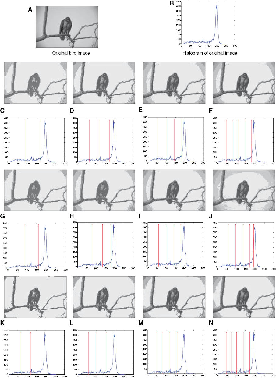
Results of Bird Image Using the HS Algorithm.
(A) Original bird image, (B) histogram of original image, (C–F) two-level to five-level thresholding-based segmented image with the best thresholds obtained from the HS algorithm using Kapur’s entropy criterion, (G–J) two-level to five-level corresponding histogram labeled with the best threshold values obtained from the HS algorithm based on the between-class variance criterion, (K–N) two-level to five-level thresholding-based segmented image with the best thresholds obtained from the HS algorithm using Tsallis entropy criterion.

Results of 86010 Image Using the HS Algorithm.
(A) Original 86010 image, (B) histogram of original image, (C–F) two-level to five-level thresholding-based segmented image with the best thresholds obtained from the HS algorithm using Kapur’s entropy criterion, (G–J) two-level to five-level corresponding histogram labeled with the best threshold values obtained from the HS algorithm based on the between-class variance criterion, (K–N) two-level to five-level thresholding-based segmented image with the best thresholds obtained from the HS algorithm using Tsallis entropy criterion.

Results of Woman Image Using the HS Algorithm.
(A) Original woman image, (B) histogram of original image, (C–F) two-level to five-level thresholding-based segmented image with the best thresholds obtained from the HS algorithm using Kapur’s entropy criterion, (G–J) two-level to five-level corresponding histogram labeled with the best threshold values obtained from the HS algorithm based on the between-class variance criterion, (K–N) two-level to five-level thresholding-based segmented image with the best thresholds obtained from the HS algorithm using Tsallis entropy criterion.
As the real-time applications need less running time in addition to high performance, the CPU time of each algorithm using Kapur’s entropy, between-class variance, and Tsallis entropy has been examined. The computation time for each evolutionary algorithm are listed in Tables 6–8, respectively. As indicated in these tables, computation time increases significantly as the threshold level increases. From these tables, it can be seen that algorithms based on between-class variance give the lowest CPU time. The results suggest that the BFO algorithm converges slowly, and the GA algorithm is the faster over all algorithms. We show also that the HS algorithm is scalable and that the running times of the algorithm seem to grow at a linear rate as the problem size increases.
4.2 Stability of Different Optimal Methods, With M = 2, 3, 4, 5
To analyze the efficiency and the stability of the algorithms, the mean and standard deviations of 35 runs for each objective function are presented in Tables 9–11. The mean μ and standard deviation σ are defined as:
The Best, Mean, and Standard Deviation of Fitness Function Values Obtained by Kapur-Based Optimization Algorithms.
| Image | M | GA | PSO | BFO | HS | ABC | |||||
|---|---|---|---|---|---|---|---|---|---|---|---|
| Mean values | STD values | Mean values | STD values | Mean values | STD values | Mean values | STD values | Mean values | STD values | ||
| 101085 | 2 | 12.82052199 | 2.8359e−02 | 12.84583123 | 3.0054e−03 | 12.84517289 | 3.9222e−03 | 12.84708191 | 9.0115e−15 | 12.84708191 | 9.0115e−15 |
| 3 | 15.89590868 | 7.4504e−02 | 15.95315876 | 1.3965e−02 | 15.93837001 | 3.3002e−02 | 15.96081266 | 5.4299e−03 | 15.96335219 | 7.9894e−05 | |
| 4 | 18.79697367 | 1.0375e−01 | 18.94790388 | 9.0562e−02 | 18.93878811 | 1.1407e−01 | 19.01366556 | 3.6046e−15 | 19.01366556 | 3.6046e−15 | |
| 5 | 21.46839312 | 1.5845e−01 | 21.58767826 | 2.2328e−01 | 21.61040088 | 1.1957e−01 | 21.74115536 | 2.6491e−03 | 21.74421953 | 7.1273e−04 | |
| Wherry | 2 | 12.15303908 | 3.7110e−02 | 12.17604958 | 7.9397e−03 | 12.17726136 | 7.4561e−04 | 12.17769204 | 1.0814e−14 | 12.17769204 | 1.0814e−14 |
| 3 | 15.04614776 | 5.7512e−02 | 15.12437386 | 2.1218e−02 | 15.11348656 | 3.7017e−02 | 15.14144981 | 1.5085e−03 | 15.14171160 | 9.0115e−15 | |
| 4 | 17.80540200 | 6.4345e−02 | 17.90540933 | 8.1410e−02 | 17.84287532 | 9.6233e−02 | 18.00449287 | 5.6352e−04 | 18.00465138 | 0.0000 | |
| 5 | 20.46041244 | 1.3367e−01 | 20.47924726 | 1.7394e−01 | 20.47257025 | 1.1209e−01 | 20.69465476 | 2.1249e−03 | 20.69614435 | 6.0005e−04 | |
| Snake | 2 | 12.35508889 | 4.2193e−02 | 12.38458786 | 8.9086e−04 | 12.38361416 | 2.5109e−03 | 12.38516237 | 9.0115e−15 | 12.38516237 | 9.0115e−15 |
| 3 | 15.46618203 | 9.5839e−02 | 15.55933284 | 1.0088e−02 | 15.54884174 | 1.8697e−02 | 15.56911780 | 1.2616e−14 | 15.56911780 | 1.2616e−14 | |
| 4 | 18.33524220 | 1.3709e−01 | 18.46398557 | 5.0500e−02 | 18.43450838 | 1.0573e−01 | 18.50563695 | 1.3089e−04 | 18.50576754 | 3.5025e−05 | |
| 5 | 20.97482075 | 1.7652e−01 | 21.01679066 | 2.3593e−01 | 21.00994809 | 1.2891e−01 | 21.21935564 | 2.6519e−03 | 21.22213439 | 1.1098e−03 | |
| Zebra | 2 | 12.19084405 | 6.4763e−02 | 12.25553412 | 3.1873e−03 | 12.24294002 | 1.4160e−02 | 12.25845978 | 1.8023e−15 | 12.25845978 | 1.8023e−15 |
| 3 | 15.21641548 | 8.8548e−02 | 15.31521544 | 3.8442e−02 | 15.28715722 | 1.5450e−02 | 15.33831416 | 3.6046e−15 | 15.33831416 | 3.6046e−15 | |
| 4 | 17.97980812 | 1.2115e−01 | 18.08345468 | 7.1347e−02 | 18.12284101 | 6.0147e−02 | 18.16887000 | 9.6622e−03 | 18.17924768 | 3.6046e−15 | |
| 5 | 20.57266710 | 1.9029e−01 | 20.76749283 | 1.7872e−01 | 20.77268838 | 1.0913e−01 | 20.99670790 | 2.0986e−04 | 20.99674337 | 7.2092e−15 | |
| Butterfly | 2 | 12.65869966 | 4.2193e−02 | 12.68280653 | 1.0218e−03 | 12.67849863 | 6.1895e−03 | 12.68395909 | 9.0115e−15 | 12.68395909 | 9.0115e−15 |
| 3 | 15.70016423 | 9.5839e−02 | 15.79376866 | 9.0072e−03 | 15.78825039 | 2.8347e−02 | 15.80151406 | 2.9681e−04 | 15.80176741 | 1.8023e−15 | |
| 4 | 18.58960198 | 1.3709e−01 | 18.74951698 | 8.3358e−02 | 18.72055629 | 8.1618e−02 | 18.80421993 | 7.2092e−15 | 18.80421993 | 7.2092e−15 | |
| 5 | 21.18151041 | 1.7652e−01 | 21.28260860 | 2.1134e−01 | 21.29588530 | 5.7040e−02 | 21.47748182 | 4.2979e−03 | 21.48227537 | 8.1304e−04 | |
| Bird | 2 | 12.06744706 | 6.4763e−02 | 12.08802639 | 4.6864e−04 | 12.08596767 | 6.4333e−03 | 12.08836104 | 2.8089e−04 | 12.08843694 | 5.4069e−15 |
| 3 | 15.07668703 | 8.8548e−02 | 15.18738613 | 1.4975e−02 | 15.18096040 | 1.6986e−02 | 15.19896385 | 0.0000 | 15.19896385 | 0.0000 | |
| 4 | 17.81901346 | 1.2115e−01 | 17.95616383 | 2.7384e−02 | 17.94890867 | 1.4248e−02 | 17.98133078 | 1.0827e−03 | 17.98259511 | 8.2385e−05 | |
| 5 | 20.30584723 | 1.9029e−01 | 20.37142389 | 2.4438e−01 | 20.37446361 | 1.8397e−01 | 20.60359095 | 5.4523e−04 | 20.60401183 | 1.3332e−04 | |
| Landscape | 2 | 11.51006157 | 4.0292e−02 | 11.54916818 | 6.7495e−03 | 11.55085540 | 1.1155e−03 | 11.55130425 | 9.0115e−15 | 11.55130425 | 9.0115e−15 |
| 3 | 14.37339605 | 1.1754e−01 | 14.45046142 | 4.7811e−02 | 14.44930759 | 2.0120e−02 | 14.51556853 | 1.0092e−03 | 14.51571143 | 1.6376e−04 | |
| 4 | 17.05431145 | 1.0296e−01 | 17.18709939 | 1.2675e−01 | 17.12897259 | 1.0431e−01 | 17.32920654 | 0.0000 | 17.32920654 | 0.0000 | |
| 5 | 19.50111564 | 1.8341e−01 | 19.52438926 | 2.7615e−01 | 19.56373127 | 1.5296e−01 | 19.90352121 | 1.1960e−02 | 19.91175226 | 2.2288e−04 | |
| Ostrich | 2 | 12.27299108 | 3.7674e−02 | 12.35150072 | 6.3101e−02 | 12.33967614 | 8.3363e−02 | 12.37287657 | 7.2092e−15 | 12.37287657 | 7.2092e−15 |
| 3 | 15.27642761 | 7.7389e−02 | 15.45180287 | 1.6694e−02 | 15.39977268 | 9.7116e−02 | 15.46610625 | 1.2854e−04 | 15.46615176 | 9.0115e−15 | |
| 4 | 17.96500933 | 1.2190e−01 | 18.02787048 | 1.2412e−01 | 18.10048771 | 2.8778e−02 | 18.13702098 | 2.3884e−03 | 18.13898333 | 2.2795e−04 | |
| 5 | 20.50001912 | 2.2370e−01 | 20.57371858 | 1.5991e−01 | 20.55920389 | 9.9762e−02 | 20.79918138 | 1.7680e−02 | 20.80473986 | 7.6301e−04 | |
| 86016 | 2 | 11.47672354 | 8.6621e−02 | 11.51607075 | 5.9495e−04 | 11.51557667 | 1.6505e−03 | 11.51653374 | 3.6046e−15 | 11.51653374 | 3.6046e−15 |
| 3 | 14.11683481 | 1.0990e−01 | 14.21005963 | 7.0464e−03 | 14.20351283 | 2.3007e−02 | 14.21639503 | 7.2092e−15 | 14.21639503 | 7.2092e−15 | |
| 4 | 16.57705139 | 1.1601e−01 | 16.64247816 | 8.8696e−02 | 16.67283490 | 5.3986e−02 | 16.70258060 | 1.8107e−03 | 16.70412197 | 7.2092e−15 | |
| 5 | 18.86065680 | 1.6979e−01 | 18.90855093 | 1.2688e−01 | 18.94008434 | 9.8987e−02 | 19.03742947 | 1.2062e−02 | 19.04966903 | 1.6809e−04 | |
| Baboon | 2 | 12.17419438 | 2.5380e−02 | 12.19573443 | 1.6782e−03 | 12.19535014 | 4.5921e−03 | 12.19611987 | 1.8710e−05 | 12.19613319 | 5.4069e−15 |
| 3 | 15.14962641 | 6.3201e−02 | 15.21669067 | 1.8323e−02 | 15.19893717 | 3.9751e−02 | 15.22290566 | 1.8593e−04 | 15.22309422 | 3.6046e−15 | |
| 4 | 17.88635194 | 7.0055e−02 | 17.97008507 | 6.8945e−02 | 17.89835904 | 9.6202e−02 | 18.01348684 | 9.3131e−04 | 18.01438333 | 2.8964e−04 | |
| 5 | 20.38959380 | 2.2099e−01 | 20.51126459 | 1.3561e−01 | 20.55199055 | 7.5954e−02 | 20.65360344 | 8.0151e−04 | 20.65397641 | 2.3340e−04 | |
| Lake | 2 | 12.42673424 | 2.7331e−02 | 12.44962185 | 4.7934e−04 | 12.44824421 | 1.0103e−02 | 12.45008781 | 5.4069e−15 | 12.45008781 | 5.4069e−15 |
| 3 | 15.35949319 | 6.9135e−02 | 15.45539618 | 1.2938e−02 | 15.45336886 | 2.3068e−02 | 15.46366271 | 9.0115e−15 | 15.46366271 | 9.0115e−15 | |
| 4 | 18.08709636 | 1.0080e−01 | 18.18419351 | 9.6761e−02 | 18.14677418 | 2.7678e−02 | 18.24438873 | 6.3402e−04 | 18.24493715 | 1.6980e−04 | |
| 5 | 20.62179165 | 1.4702e−01 | 20.66385658 | 2.3620e−01 | 20.72985762 | 3.4766e−02 | 20.87909950 | 4.8462e−03 | 20.88088882 | 4.4570e−04 | |
| Women | 2 | 12.62914177 | 4.0400e−02 | 12.66030605 | 4.4834e−03 | 12.66121382 | 1.0905e−03 | 12.66160897 | 1.8023e−15 | 12.66160897 | 1.8023e−15 |
| 3 | 15.65140351 | 6.2439e−02 | 15.72726721 | 2.9291e−02 | 15.73375176 | 5.6686e−03 | 15.73837768 | 4.7575e−05 | 15.73843511 | 1.2616e−14 | |
| 4 | 18.40413565 | 1.0430e−01 | 18.49225411 | 8.7040e−02 | 18.48832431 | 3.5122e−02 | 18.54473415 | 2.3362e−03 | 18.54600454 | 6.6336e−05 | |
| 5 | 21.00683579 | 1.1359e−01 | 21.01124763 | 2.8521e−01 | 21.09320652 | 5.1418e−02 | 21.22008847 | 4.8344e−03 | 21.22319221 | 3.4335e−04 | |
The Best, Mean and Standard Deviation of Fitness Function Values Obtained by Between-Class Variance-Based Optimization Algorithms.
| Image | M | GA | PSO | BFO | HS | ABC | |||||
|---|---|---|---|---|---|---|---|---|---|---|---|
| Mean values | STD values | Mean values | STD values | Mean values | STD values | Mean values | STD values | Mean values | STD values | ||
| 101085 | 2 | 2747.41775937 | 8.0044e+00 | 2755.59969607 | 8.7606e−01 | 2753.22929383 | 8.3490e+00 | 2755.80780607 | 1.3842e−12 | 2755.80780607 | 1.3842e−12 |
| 3 | 2933.62190136 | 1.8614e+01 | 2959.57489747 | 2.8494e+00 | 2956.77694513 | 1.0433e+01 | 2960.76326610 | 7.1861e−03 | 2960.77194057 | 1.3842e−12 | |
| 4 | 3038.59954401 | 1.4014e+01 | 3055.30599815 | 1.3010e+01 | 3049.07127475 | 7.4326e+00 | 3063.49903906 | 3.5467e−03 | 3063.49963857 | 4.6139e−13 | |
| 5 | 3090.23750950 | 1.8063e+01 | 3105.26155364 | 1.1863e+01 | 3101.35871708 | 8.6588e+00 | 3115.46282647 | 3.4656e−01 | 3115.73528570 | 2.8522e−02 | |
| Wherry | 2 | 3062.63168600 | 2.5984e+01 | 3082.21891963 | 6.2883e+00 | 3083.61927775 | 7.4872e−01 | 3083.79418431 | 2.3069e−12 | 3083.79418431 | 2.3069e−12 |
| 3 | 3294.09730404 | 3.4371e+01 | 3322.35869963 | 8.4946e+00 | 3311.31486572 | 3.7967e+01 | 3326.67830302 | 0.0000 | 3326.67830302 | 0.0000 | |
| 4 | 3362.80240224 | 2.1296e+01 | 3384.75222691 | 1.1162e+01 | 3370.59941547 | 1.1761e+01 | 3390.47774580 | 6.1928e−03 | 3390.47928530 | 1.3842e−12 | |
| 5 | 3397.34466483 | 1.4069e+01 | 3404.54457081 | 1.5054e+01 | 3401.91683478 | 8.4337e+00 | 3422.61828203 | 6.3124e−01 | 3422.86962679 | 2.0165e−02 | |
| Snake | 2 | 1100.08492317 | 1.0442e+01 | 1109.80532807 | 4.6743e−01 | 1109.99888917 | 4.7743e−02 | 1109.97605290 | 4.6139e−13 | 1110.02017316 | 6.9208e−13 |
| 3 | 1204.63961698 | 1.2847e+01 | 1218.20058577 | 3.4950e+00 | 1217.71739055 | 3.5976e+00 | 1219.84832870 | 8.0743e−13 | 1219.84832870 | 2.3069e−13 | |
| 4 | 1255.37007501 | 1.2502e+01 | 1268.10107713 | 8.7244e+00 | 1270.25826403 | 1.0780e+01 | 1274.27631654 | 1.1580e−02 | 1274.29104142 | 1.1535e−12 | |
| 5 | 1281.46261481 | 1.2303e+01 | 1291.80675694 | 1.1693e+01 | 1291.38926856 | 9.2023e+00 | 1303.62901862 | 1.6921e−01 | 1303.75797217 | 3.5298e−02 | |
| Zebra | 2 | 805.43768318 | 1.4347e+01 | 817.30914065 | 1.2563e+00 | 816.02235882 | 3.6195e+00 | 817.64291521 | 1.8455e−12 | 817.64291521 | 4.6139e−13 |
| 3 | 896.30139737 | 1.7342e+01 | 911.73953478 | 1.1489e+01 | 910.12497126 | 7.1447e+00 | 915.10304297 | 1.2370e−02 | 915.10304297 | 8.0743e−13 | |
| 4 | 948.90555841 | 1.1229e+01 | 956.68814919 | 1.3499e+01 | 951.61717954 | 5.2185e+00 | 964.93185053 | 8.1686e−01 | 964.93580002 | 6.8215e−04 | |
| 5 | 973.48105242 | 8.9206e+00 | 978.78211447 | 1.3223e+01 | 982.71600707 | 4.2504e+00 | 989.84854555 | 2.7180e−02 | 990.02687776 | 2.6965e−02 | |
| Butterfly | 2 | 3501.12996183 | 1.9504e+01 | 3519.16766370 | 3.0427e−01 | 3518.45013486 | 3.6278e+00 | 3519.36925589 | 1.2747e−12 | 3519.36925589 | 1.8455e−12 |
| 3 | 3618.53520443 | 2.0398e+01 | 3642.96555490 | 8.5487e+00 | 3642.31940939 | 1.2444e+01 | 3646.00742166 | 0.0000 | 3646.01996751 | 0.0000 | |
| 4 | 3694.21873999 | 1.0996e+01 | 3698.49843997 | 2.0868e+01 | 3707.99253277 | 3.3170e+00 | 3711.32977088 | 2.8215e−02 | 3712.04921273 | 1.5745e−02 | |
| 5 | 3729.68994546 | 1.7317e+01 | 3738.90865383 | 1.6254e+01 | 3745.94094974 | 1.0035e+01 | 3760.31932153 | 9.6896e−01 | 3760.33280358 | 1.1099e−02 | |
| Bird | 2 | 2524.91739451 | 1.5737e+01 | 2535.41355510 | 6.5092e−02 | 2534.74116703 | 3.8534e+00 | 2535.43896987 | 1.8455e−12 | 2535.45049890 | 4.6139e−13 |
| 3 | 2600.33061881 | 7.7778e+00 | 2610.64307969 | 3.1857e+00 | 2607.80984795 | 8.2055e+00 | 2611.87729789 | 0.0000 | 2611.87729789 | 0.0000 | |
| 4 | 2636.50152285 | 8.4040e+00 | 2644.05617678 | 9.4044e+00 | 2643.76030179 | 3.9022e+00 | 2649.66137434 | 6.8165e−02 | 2649.68644784 | 0.0000 | |
| 5 | 2655.60078232 | 8.6270e+00 | 2658.08594368 | 1.0564e+01 | 2664.70084429 | 2.4394e+00 | 2667.72263525 | 6.7924e−03 | 2668.30678984 | 2.5704e−02 | |
| Landscape | 2 | 4404.21199755 | 1.5824e+01 | 4419.73105790 | 1.1659e−01 | 4415.78053596 | 9.7574e+00 | 4419.79062113 | 2.3069e−13 | 4419.79062113 | 1.8455e−12 |
| 3 | 4680.25519778 | 2.9967e+01 | 4718.18006349 | 9.7768e+00 | 4718.90749524 | 1.2832e+00 | 4721.18853555 | 6.0303e−02 | 4721.18853555 | 0.0000 | |
| 4 | 4764.41623385 | 1.7009e+01 | 4778.94613134 | 1.2416e+01 | 4780.14196584 | 3.1896e+00 | 4783.75030895 | 4.5076e−01 | 4783.78331215 | 3.6911e−12 | |
| 5 | 4799.33406144 | 1.5701e+01 | 4814.05357097 | 1.4490e+01 | 4817.76327821 | 7.4472e+00 | 4823.80226355 | 1.8507e−01 | 4823.80426574 | 3.6911e−12 | |
| Ostrich | 2 | 1019.03567856 | 2.0916e+01 | 1035.21639397 | 8.3050e−01 | 1035.39827725 | 9.7406e−02 | 1035.42809860 | 4.6139e−13 | 1035.42809860 | 2.3069e−13 |
| 3 | 1083.35223898 | 2.1069e+01 | 1096.44126535 | 5.4144e+00 | 1093.73881239 | 9.9347e+00 | 1099.34543867 | 5.7429e−02 | 1099.38285377 | 9.2277e−13 | |
| 4 | 1128.88736365 | 9.9764e+00 | 1131.03106777 | 1.2328e+01 | 1129.92852266 | 9.3165e+00 | 1139.83637174 | 2.0638e−02 | 1139.96812598 | 7.3686e−03 | |
| 5 | 1149.81073146 | 1.1479e+01 | 1155.50362778 | 1.3927e+01 | 1153.04209857 | 6.8833e+00 | 1168.56966515 | 2.4331e−01 | 1168.69833858 | 2.8236e−02 | |
| 86016 | 2 | 1227.82985739 | 1.0181e+01 | 1236.52027265 | 6.7109e−01 | 1236.69285132 | 7.8639e−02 | 1236.70799926 | 3.4879e−08 | 1236.70799926 | 4.6139e−13 |
| 3 | 1280.93837534 | 9.4973e+00 | 1289.38689188 | 9.7991e−01 | 1287.11324934 | 7.6140e+00 | 1289.92795608 | 2.5285e−02 | 1289.94189074 | 6.9208e−13 | |
| 4 | 1312.93511530 | 6.7801e+00 | 1318.13306170 | 5.8807e+00 | 1315.18483812 | 4.6107e+00 | 1321.72165141 | 1.2137e−02 | 1321.74260380 | 4.6139e−13 | |
| 5 | 1327.55307056 | 6.4192e+00 | 1331.24127703 | 6.4873e+00 | 1331.21688226 | 4.3156e+00 | 1337.10135969 | 8.3182e−02 | 1337.33642824 | 2.7948e−02 | |
| Baboon | 2 | 1529.85593415 | 1.2920e+01 | 1539.43786300 | 1.7374e+00 | 1539.47509013 | 2.1947e+00 | 1539.79837114 | 2.3069e−12 | 1539.84605676 | 1.1535e−12 |
| 3 | 1618.00628033 | 1.0895e+01 | 1628.45525245 | 8.9986e−01 | 1623.79318366 | 9.4415e+00 | 1629.35169000 | 1.7050e−02 | 1629.37795050 | 0.0000 | |
| 4 | 1662.75942230 | 1.3284e+01 | 1673.76768446 | 1.3519e+01 | 1677.81465797 | 5.5326e+00 | 1682.64963934 | 3.9298e−02 | 1682.66934400 | 4.5382e−03 | |
| 5 | 1688.93571424 | 1.4031e+01 | 1697.84174402 | 9.6949e+00 | 1696.41215387 | 7.8716e+00 | 1707.90231800 | 3.6480e−02 | 1708.19209379 | 2.9005e−02 | |
| Lake | 2 | 3730.64835091 | 1.6479e+01 | 3741.23824487 | 1.6949e−01 | 3741.31255700 | 8.5346e−02 | 3741.31365506 | 2.3069e−12 | 3741.34541715 | 1.3842e−12 |
| 3 | 3853.78580682 | 1.7915e+01 | 3875.47791295 | 4.1545e+00 | 3875.35963709 | 3.0227e+00 | 3876.94607225 | 2.3069e−12 | 3876.94624749 | 1.3842e−12 | |
| 4 | 3919.90727096 | 1.8419e+01 | 3936.96356987 | 1.2028e+01 | 3937.02703424 | 8.8277e+00 | 3943.25561280 | 2.3629e−01 | 3943.26884069 | 2.3069e−12 | |
| 5 | 3954.84240661 | 1.3661e+01 | 3960.85952971 | 1.7562e+01 | 3960.79458569 | 7.1800e+00 | 3977.28048204 | 2.7131e−03 | 3977.34358202 | 9.8343e−04 | |
| Women | 2 | 2604.638195 | 2.1537e+01 | 2604.14614498 | 2.1231e+00 | 2604.43730801 | 8.2807e−01 | 2604.63819548 | 1.8455e−12 | 2604.63819548 | 1.8455e−12 |
| 3 | 2780.762981 | 2.6052e+01 | 2778.12186584 | 9.4845e+00 | 2777.12557345 | 9.6898e+00 | 2780.77911258 | 1.3842e−12 | 2780.77911258 | 1.3842e−12 | |
| 4 | 2849.065166 | 1.6122e+01 | 2844.44048838 | 1.1638e+01 | 2839.55301955 | 5.6739e+00 | 2851.72103650 | 8.5253e−02 | 2851.78138263 | 1.9963e−02 | |
| 5 | 2882.946131 | 1.6031e+01 | 2868.66237510 | 1.7940e+01 | 2877.32055889 | 1.2368e+01 | 2886.28052907 | 3.4555e−01 | 2886.42604510 | 3.5532e−02 | |
The Best, Mean, and Standard Deviation of Fitness Function Values Obtained by Tsallis-Based Optimization Algorithms.
| Image | M | GA | PSO | BFO | HS | ABC | |||||
|---|---|---|---|---|---|---|---|---|---|---|---|
| Mean values | STD values | Mean values | STD values | Mean values | STD values | Mean values | STD values | Mean values | STD values | ||
| 101085 | 2 | 0.88888340 | 1.5189e−06 | 0.88888449 | 1.3128e−07 | 0.88888450 | 1.2522e−07 | 0.88888454 | 0.000000 | 0.88888454 | 0.0000 |
| 3 | 1.29626985 | 4.7905e−06 | 1.29627569 | 8.5467e−07 | 1.29627569 | 1.2244e−06 | 1.29627626 | 2.0534e−09 | 1.29627626 | 4.5057e−16 | |
| 4 | 1.65425878 | 1.6277e−05 | 1.65427295 | 5.7070e−06 | 1.65425618 | 1.6011e−05 | 1.65427731 | 2.3359e−08 | 1.65427731 | 9.0115e−16 | |
| 5 | 1.99571251 | 6.2935e−05 | 1.99574784 | 7.4098e−05 | 1.99573238 | 1.1691e−04 | 1.99579544 | 2.2544e−07 | 1.99579571 | 1.4426e−07 | |
| Wherry | 2 | 0.88886740 | 5.3247e−06 | 0.88887289 | 2.5928e−07 | 0.88887296 | 8.7936e−08 | 0.88887305 | 0.000000 | 0.88887305 | 0.000000 |
| 3 | 1.29620159 | 4.3955e−05 | 1.29623189 | 3.2039e−06 | 1.29621824 | 1.0368e−05 | 1.29623483 | 6.7586e−16 | 1.29623483 | 6.7586e−16 | |
| 4 | 1.65411092 | 5.3992e−05 | 1.65415705 | 2.9189e−05 | 1.65414289 | 4.0287e−05 | 1.65417714 | 1.7788e−06 | 1.65417873 | 6.6898e−08 | |
| 5 | 1.99543743 | 1.8458e−04 | 1.99548952 | 1.9044e−04 | 1.99551089 | 1.6146e−04 | 1.99565696 | 5.9424e−06 | 1.99565860 | 1.0684e−07 | |
| Snake | 2 | 0.88888181 | 3.3345e−07 | 0.88888211 | 2.1207e−08 | 0.88888206 | 3.6556e−08 | 0.88888212 | 3.3793e−16 | 0.88888212 | 3.3793e−16 |
| 3 | 1.29627444 | 3.7883e−06 | 1.29627813 | 9.4122e−07 | 1.29627757 | 7.3879e−07 | 1.29627868 | 9.0115e−16 | 1.29627868 | 9.0115e−16 | |
| 4 | 1.65426928 | 9.6244e−06 | 1.65427468 | 1.0835e−05 | 1.65427633 | 4.3316e−06 | 1.65428073 | 2.7678e−08 | 1.65428075 | 1.5770e−15 | |
| 5 | 1.99577377 | 2.3209e−05 | 1.99578533 | 3.9213e−05 | 1.99579416 | 1.0011e−05 | 1.99580931 | 5.8628e−07 | 1.99580980 | 9.7110e−08 | |
| Zebra | 2 | 0.88887927 | 2.2132e−06 | 0.88888114 | 9.7922e−08 | 0.88888105 | 4.5131e−07 | 0.88888123 | 6.7586e−16 | 0.88888123 | 6.7586e−16 |
| 3 | 1.29625553 | 1.1570e−05 | 1.29626751 | 1.3878e−06 | 1.29626443 | 5.4213e−06 | 1.29626862 | 4.5057e−16 | 1.29626862 | 4.5057e−16 | |
| 4 | 1.65421618 | 2.1955e−05 | 1.65423418 | 1.3341e−05 | 1.65421934 | 1.9017e−05 | 1.65424610 | 2.6210e−06 | 1.65424683 | 4.5057e−16 | |
| 5 | 1.99562319 | 9.6830e−05 | 1.99568540 | 7.2716e−05 | 1.99568869 | 2.8146e−05 | 1.99574598 | 1.7186e−06 | 1.99574708 | 8.1398e−08 | |
| Butterfly | 2 | 0.88888494 | 4.3446e−07 | 0.88888522 | 4.5792e−08 | 0.88888518 | 1.2222e−07 | 0.88888526 | 2.1098e−08 | 0.88888526 | 3.3793e−16 |
| 3 | 1.29627793 | 6.9310e−06 | 1.29628377 | 2.5366e−07 | 1.29628349 | 1.3947e−06 | 1.29628414 | 0.000000 | 1.29628414 | 0.000000 | |
| 4 | 1.65427310 | 1.0294e−05 | 1.65427837 | 1.2865e−05 | 1.65427360 | 1.0379e−05 | 1.65428486 | 8.8394e−07 | 1.65428512 | 4.5057e−16 | |
| 5 | 1.99574248 | 7.6556e−05 | 1.99578810 | 5.2309e−05 | 1.99578129 | 2.8925e−05 | 1.99581637 | 1.3700e−06 | 1.99581673 | 3.9199e−08 | |
| Bird | 2 | 0.88886956 | 1.5951e−06 | 0.88887099 | 1.5864e−08 | 0.88887046 | 1.2285e−06 | 0.88887099 | 2.2529e−16 | 0.88887099 | 2.2529e−16 |
| 3 | 1.29624736 | 5.3968e−06 | 1.29625263 | 8.3063e−07 | 1.29625264 | 6.8679e−07 | 1.29625326 | 2.8086e−10 | 1.29625326 | 6.7586e−16 | |
| 4 | 1.65422188 | 2.0183e−05 | 1.65423333 | 1.7750e−05 | 1.65423838 | 8.0094e−06 | 1.65424292 | 4.9124e−07 | 1.65424329 | 6.7586e−16 | |
| 5 | 1.99566981 | 1.0552e−04 | 1.99570021 | 8.0978e−05 | 1.99572015 | 2.3724e−05 | 1.99575107 | 6.1590e−07 | 1.99575152 | 3.8657e−07 | |
| Landscape | 2 | 0.88884579 | 5.6849e−06 | 0.88885023 | 1.3611e−06 | 0.88884920 | 5.7021e−06 | 0.88885058 | 1.1264e−16 | 0.88885058 | 1.1264e−16 |
| 3 | 1.29616205 | 1.5625e−05 | 1.29618020 | 6.3769e−06 | 1.29616884 | 1.3362e−05 | 1.29618603 | 6.7586e−16 | 1.29618603 | 6.7586e−16 | |
| 4 | 1.65405517 | 6.9574e−05 | 1.65409365 | 2.1020e−05 | 1.65407412 | 5.2155e−05 | 1.65413205 | 1.0698e−05 | 1.65413469 | 2.7631e−09 | |
| 5 | 1.99527685 | 2.5657e−04 | 1.99541732 | 2.4740e−04 | 1.99542159 | 1.9204e−04 | 1.99557992 | 1.9889e−07 | 1.99558005 | 1.2605e−08 | |
| Ostrich | 2 | 0.88887998 | 1.6353e−06 | 0.88888172 | 2.6141e−07 | 0.88888153 | 6.6187e−07 | 0.88888197 | 0.000000 | 0.88888197 | 0.000000 |
| 3 | 1.29626353 | 1.4416e−05 | 1.29627481 | 1.4311e−06 | 1.29626982 | 1.1177e−05 | 1.29627608 | 4.5057e−16 | 1.29627608 | 4.5057e−16 | |
| 4 | 1.65423049 | 2.1910e−05 | 1.65424283 | 1.9686e−05 | 1.65425037 | 8.1890e−06 | 1.65425586 | 1.4422e−06 | 1.65425696 | 4.5057e−16 | |
| 5 | 1.99565232 | 6.1718e−05 | 1.99570715 | 8.2812e−05 | 1.99573640 | 1.9323e−05 | 1.99577160 | 2.6914e−07 | 1.99577169 | 2.5633e−08 | |
| 86016 | 2 | 0.88887575 | 2.2775e−06 | 0.88887762 | 7.4559e−08 | 0.88887755 | 1.6397e−07 | 0.88887766 | 3.3793e−16 | 0.88887766 | 3.3793e−16 |
| 3 | 1.29623418 | 1.5029e−05 | 1.29624563 | 7.1138e−06 | 1.29624794 | 1.8802e−06 | 1.29624958 | 0.000000 | 1.29624958 | 0.000000 | |
| 4 | 1.65416521 | 3.5282e−05 | 1.65418275 | 5.0246e−05 | 1.65419780 | 1.4510e−05 | 1.65421297 | 9.0115e−16 | 1.65421297 | 9.0115e−16 | |
| 5 | 1.99551704 | 1.1625e−04 | 1.99553275 | 1.4827e−04 | 1.99561600 | 2.2566e−05 | 1.99566589 | 2.3373e−06 | 1.99566695 | 3.2370e−08 | |
| Baboon | 2 | 0.88888329 | 9.5040e−07 | 0.88888387 | 2.4052e−08 | 0.88888387 | 3.9486e−09 | 0.88888388 | 4.5057e−16 | 0.88888388 | 4.5057e−16 |
| 3 | 1.29627032 | 1.0629e−05 | 1.29627653 | 5.7277e−07 | 1.29627532 | 2.0892e−06 | 1.29627690 | 6.7586e−16 | 1.29627690 | 6.7586e−16 | |
| 4 | 1.65425889 | 1.1422e−05 | 1.65426520 | 1.2979e−05 | 1.65425582 | 1.0554e−05 | 1.65427298 | 8.8313e−08 | 1.65427304 | 1.2521e−08 | |
| 5 | 1.99571548 | 6.7792e−05 | 1.99575063 | 7.4421e−05 | 1.99576301 | 1.0776e−05 | 1.99578983 | 3.3858e−07 | 1.99579007 | 7.3425e−08 | |
| Lake | 2 | 0.88888359 | 3.5804e−07 | 0.88888387 | 1.2823e−08 | 0.88888386 | 7.6242e−08 | 0.88888388 | 3.3793e−16 | 0.88888388 | 3.3793e−16 |
| 3 | 1.29627237 | 6.3097e−06 | 1.29627795 | 1.7305e−06 | 1.29627797 | 5.2360e−07 | 1.29627861 | 6.7377e−09 | 1.29627861 | 4.5057e−16 | |
| 4 | 1.65426204 | 1.0584e−05 | 1.65426956 | 6.2208e−06 | 1.65426170 | 2.7868e−05 | 1.65427497 | 1.2837e−06 | 1.65427595 | 4.9646e−09 | |
| 5 | 1.99572075 | 5.1393e−05 | 1.99573879 | 1.0328e−04 | 1.99576707 | 2.7981e−05 | 1.99579722 | 4.7955e−07 | 1.99579742 | 5.9907e−08 | |
| Women | 2 | 0.88888568 | 4.2045e−07 | 0.88888602 | 3.5371e−08 | 0.88888600 | 1.3501e−07 | 0.88888604 | 5.6322e−16 | 0.88888604 | 5.6322e−16 |
| 3 | 1.29628073 | 4.5012e−06 | 1.29628465 | 1.1870e−06 | 1.29628406 | 1.2240e−06 | 1.29628496 | 1.5216e−10 | 1.29628496 | 6.7586e−16 | |
| 4 | 1.65427971 | 9.1184e−06 | 1.65428749 | 6.5003e−06 | 1.65428523 | 1.5216e−05 | 1.65429046 | 2.3453e−07 | 1.65429055 | 2.2901e−09 | |
| 5 | 1.99576913 | 3.3826e−05 | 1.99578698 | 3.6372e−05 | 1.99580015 | 1.4672e−05 | 1.99582141 | 7.9136e−07 | 1.99582209 | 5.5821e−08 | |
where k is the number of runs for each stochastic algorithm (k = 30), σi is the best objective value obtained by the ith run of the algorithm.
From Tables 9–11, it can be seen that the variance values increase with the increasing numbers of the threshold; that is to say, the stability of the algorithms declines with the increasing number of the threshold. We can observe that the variance of HS and ABC are smaller than the variance of BFO, GA, and PSO algorithms for all the number of thresholds and for all images. The numerical results in Tables 9–11 indicate that for some images, the HS algorithm seems to be more sensible to the increase in the number of thresholds than the ABC algorithm.
A nonparametric statistical test known as the Wilcoxon’s rank sum test for independent samples [12, 35] has been conducted, with a 5% significance level to test if the algorithms used in this study have equal median values using between-class variance, Kapur or Tsallis entropy.
In the first experiment, the HS algorithm was chosen as the control algorithm and was compared with the GA, PSO, and BFO algorithms in terms of the mean value for each objective function. The number of cases investigated is 48 × 35 runs have been analyzed in total.
Table 12 reports the p-values produced by Wilcoxon’s test for the pair-wise comparison of three groups. Such groups are constituted by HS vs.GA, HS vs. PSO, and HS vs. BFO. As a null hypothesis, it is assumed that there is no significant difference between mean values of the four algorithms. The alternative hypothesis considers a significant difference between the four algorithms.
Statistical Analysis of 35 Runs for each of 12*4 Cases for the Experiments on Each Criterion.
| Image | M | Between-class variance | Kapur’s entropy | Tsallis entropy | |||||||||||||||
|---|---|---|---|---|---|---|---|---|---|---|---|---|---|---|---|---|---|---|---|
| HS vs. GA | HS vs. PSO | HS vs. BFO | HS vs. GA | HS vs. PSO | HS vs. BFO | HS vs. GA | HS vs. PSO | HS vs. BFO | |||||||||||
| p-Value | H | p-Value | H | p-Value | H | p-Value | H | p-Value | H | p-Value | H | p-Value | H | p-Value | H | p-Value | H | ||
| 101085 | 2 | 0.000000 | 1 | 0.000000 | 1 | 0.000178 | 1 | 0.000000 | 1 | 0.000000 | 1 | 0.000000 | 1 | 0.000000 | 1 | 0.000000 | 1 | 0.011469 | 1 |
| 3 | 0.000001 | 1 | 0.000001 | 1 | 0.000000 | 1 | 0.000000 | 1 | 0.000001 | 1 | 0.000000 | 1 | 0.000000 | 1 | 0.000001 | 1 | 0.000000 | 1 | |
| 4 | 0.000000 | 1 | 0.000000 | 1 | 0.000000 | 1 | 0.000000 | 1 | 0.000000 | 1 | 0.000000 | 1 | 0.000000 | 1 | 0.000000 | 1 | 0.000000 | 1 | |
| 5 | 0.000000 | 1 | 0.000000 | 1 | 0.000000 | 1 | 0.000000 | 1 | 0.000000 | 1 | 0.000000 | 1 | 0.000000 | 1 | 0.000000 | 1 | 0.000000 | 1 | |
| Wherry | 2 | 0.000000 | 1 | 0.000000 | 1 | 0.1602960 | 0.000000 | 1 | 0.000000 | 1 | 0.000084 | 1 | 0.000000 | 1 | 0.000000 | 1 | 0.000000 | 1 | |
| 3 | 0.000001 | 1 | 0.000001 | 1 | 0.000000 | 1 | 0.000000 | 1 | 0.000001 | 1 | 0.000000 | 1 | 0.000000 | 1 | 0.000001 | 1 | 0.000000 | 1 | |
| 4 | 0.000000 | 1 | 0.000000 | 1 | 0.000000 | 1 | 0.000000 | 1 | 0.000000 | 1 | 0.000000 | 1 | 0.000000 | 1 | 0.000000 | 1 | 0.000000 | 1 | |
| 5 | 0.000000 | 1 | 0.000000 | 1 | 0.000000 | 1 | 0.000000 | 1 | 0.000000 | 1 | 0.000000 | 1 | 0.000000 | 1 | 0.000000 | 1 | 0.000000 | 1 | |
| Snake | 2 | 0.000000 | 1 | 0.000000 | 1 | 0.042411 | 1 | 0.000000 | 1 | 0.000000 | 1 | 0.000082 | 1 | 0.000000 | 1 | 0.000000 | 1 | 0.000389 | 1 |
| 3 | 0.000001 | 1 | 0.000001 | 1 | 0.000000 | 1 | 0.000000 | 1 | 0.000001 | 1 | 0.000000 | 1 | 0.000000 | 1 | 0.000001 | 1 | 0.000000 | 1 | |
| 4 | 0.000000 | 1 | 0.000000 | 1 | 0.000000 | 1 | 0.000000 | 1 | 0.000000 | 1 | 0.000000 | 1 | 0.000000 | 1 | 0.000000 | 1 | 0.000008 | 1 | |
| 5 | 0.000000 | 1 | 0.000000 | 1 | 0.000000 | 1 | 0.000000 | 1 | 0.000000 | 1 | 0.000000 | 1 | 0.000000 | 1 | 0.000000 | 1 | 0.000000 | 1 | |
| Zebra | 2 | 0.000000 | 1 | 0.000000 | 1 | 0.000008 | 1 | 0.000000 | 1 | 0.000000 | 1 | 0.000000 | 1 | 0.000000 | 1 | 0.000000 | 1 | 0.000000 | 1 |
| 3 | 0.000001 | 1 | 0.000001 | 1 | 0.000000 | 1 | 0.000000 | 1 | 0.000001 | 1 | 0.000000 | 1 | 0.000000 | 1 | 0.000001 | 1 | 0.000000 | 1 | |
| 4 | 0.000000 | 1 | 0.000000 | 1 | 0.000000 | 1 | 0.000000 | 1 | 0.000000 | 1 | 0.000632 | 1 | 0.000000 | 1 | 0.000000 | 1 | 0.000000 | 1 | |
| 5 | 0.000000 | 1 | 0.000000 | 1 | 0.000000 | 1 | 0.000000 | 1 | 0.000000 | 1 | 0.000000 | 1 | 0.000000 | 1 | 0.000000 | 1 | 0.000000 | 1 | |
| Butterfly | 2 | 0.000000 | 1 | 0.000000 | 1 | 0.000003 | 1 | 0.000000 | 1 | 0.000000 | 1 | 0.000000 | 1 | 0.000000 | 1 | 0.000000 | 1 | 0.000000 | 1 |
| 3 | 0.000001 | 1 | 0.000001 | 1 | 0.000000 | 1 | 0.000000 | 1 | 0.000001 | 1 | 0.000002 | 1 | 0.000000 | 1 | 0.000001 | 1 | 0.000000 | 1 | |
| 4 | 0.000000 | 1 | 0.000000 | 1 | 0.005474 | 1 | 0.000000 | 1 | 0.000000 | 1 | 0.000000 | 1 | 0.000000 | 1 | 0.000000 | 1 | 0.000000 | 1 | |
| 5 | 0.000000 | 1 | 0.000000 | 1 | 0.000000 | 1 | 0.000000 | 1 | 0.000000 | 1 | 0.000000 | 1 | 0.000000 | 1 | 0.000000 | 1 | 0.000000 | 1 | |
| Bird | 2 | 0.000000 | 1 | 0.000000 | 1 | 0.000004 | 1 | 0.000000 | 1 | 0.000000 | 1 | 0.000063 | 1 | 0.000000 | 1 | 0.000000 | 1 | 0.000002 | 1 |
| 3 | 0.000001 | 1 | 0.000001 | 1 | 0.000000 | 1 | 0.000000 | 1 | 0.000001 | 1 | 0.000000 | 1 | 0.000000 | 1 | 0.000001 | 1 | 0.000000 | 1 | |
| 4 | 0.000000 | 1 | 0.000000 | 1 | 0.000000 | 1 | 0.000000 | 1 | 0.000000 | 1 | 0.000000 | 1 | 0.000000 | 1 | 0.000000 | 1 | 0.000000 | 1 | |
| 5 | 0.000000 | 1 | 0.000000 | 1 | 0.000000 | 1 | 0.000000 | 1 | 0.000000 | 1 | 0.000000 | 1 | 0.000000 | 1 | 0.000000 | 1 | 0.000000 | 1 | |
| Landscape | 2 | 0.000000 | 1 | 0.000000 | 1 | 0.3351790 | 0.000000 | 1 | 0.000000 | 1 | 0.021982 | 1 | 0.000000 | 1 | 0.000000 | 1 | 0.000029 | 1 | |
| 3 | 0.000001 | 1 | 0.000001 | 1 | 0.000000 | 1 | 0.000000 | 1 | 0.000001 | 1 | 0.000000 | 1 | 0.000000 | 1 | 0.000001 | 1 | 0.000000 | 1 | |
| 4 | 0.000000 | 1 | 0.000000 | 1 | 0.000000 | 1 | 0.000000 | 1 | 0.000000 | 1 | 0.000000 | 1 | 0.000000 | 1 | 0.000000 | 1 | 0.000000 | 1 | |
| 5 | 0.000000 | 1 | 0.000000 | 1 | 0.000000 | 1 | 0.000000 | 1 | 0.000000 | 1 | 0.000000 | 1 | 0.000000 | 1 | 0.000000 | 1 | 0.000000 | 1 | |
| Ostrich | 2 | 0.000000 | 1 | 0.000000 | 1 | 0.000000 | 1 | 0.000000 | 1 | 0.000000 | 1 | 0.000177 | 1 | 0.000000 | 1 | 0.000000 | 1 | 0.000000 | 1 |
| 3 | 0.000001 | 1 | 0.000001 | 1 | 0.000000 | 1 | 0.000000 | 1 | 0.000001 | 1 | 0.000000 | 1 | 0.000000 | 1 | 0.000001 | 1 | 0.000000 | 1 | |
| 4 | 0.000000 | 1 | 0.000000 | 1 | 0.000000 | 1 | 0.000000 | 1 | 0.000000 | 1 | 0.000000 | 1 | 0.000000 | 1 | 0.000000 | 1 | 0.000000 | 1 | |
| 5 | 0.000000 | 1 | 0.000000 | 1 | 0.000000 | 1 | 0.000000 | 1 | 0.000000 | 1 | 0.000000 | 1 | 0.000000 | 1 | 0.000000 | 1 | 0.000000 | 1 | |
| 86016 | 2 | 0.000000 | 1 | 0.000000 | 1 | 0.000004 | 1 | 0.000000 | 1 | 0.000000 | 1 | 0.001470 | 1 | 0.000000 | 1 | 0.000000 | 1 | 0.000000 | 1 |
| 3 | 0.000001 | 1 | 0.000001 | 1 | 0.000000 | 1 | 0.000000 | 1 | 0.000001 | 1 | 0.000000 | 1 | 0.000000 | 1 | 0.000001 | 1 | 0.000000 | 1 | |
| 4 | 0.000000 | 1 | 0.000000 | 1 | 0.000000 | 1 | 0.000000 | 1 | 0.000000 | 1 | 0.000000 | 1 | 0.000000 | 1 | 0.000000 | 1 | 0.000000 | 1 | |
| 5 | 0.000000 | 1 | 0.000000 | 1 | 0.000000 | 1 | 0.000000 | 1 | 0.000000 | 1 | 0.000000 | 1 | 0.000000 | 1 | 0.000000 | 1 | 0.000000 | 1 | |
| Baboon | 2 | 0.000000 | 1 | 0.000000 | 1 | 0.000000 | 1 | 0.000000 | 1 | 0.000000 | 1 | 0.2179420 | 0.000000 | 1 | 0.000000 | 1 | 0.000000 | 1 | |
| 3 | 0.000001 | 1 | 0.000001 | 1 | 0.000000 | 1 | 0.000000 | 1 | 0.000001 | 1 | 0.000000 | 1 | 0.000000 | 1 | 0.000001 | 1 | 0.000000 | 1 | |
| 4 | 0.000000 | 1 | 0.000000 | 1 | 0.000000 | 1 | 0.000000 | 1 | 0.000000 | 1 | 0.000000 | 1 | 0.000000 | 1 | 0.000000 | 1 | 0.000000 | 1 | |
| 5 | 0.000000 | 1 | 0.000000 | 1 | 0.000000 | 1 | 0.000000 | 1 | 0.000000 | 1 | 0.000000 | 1 | 0.000000 | 1 | 0.000000 | 1 | 0.000000 | 1 | |
| Lake | 2 | 0.000000 | 1 | 0.000000 | 1 | 0.000003 | 1 | 0.000000 | 1 | 0.000000 | 1 | 0.022093 | 1 | 0.000000 | 1 | 0.000000 | 1 | 0.000000 | 1 |
| 3 | 0.000001 | 1 | 0.000001 | 1 | 0.000000 | 1 | 0.000000 | 1 | 0.000001 | 1 | 0.000000 | 1 | 0.000000 | 1 | 0.000001 | 1 | 0.000000 | 1 | |
| 4 | 0.000000 | 1 | 0.000000 | 1 | 0.000000 | 1 | 0.000000 | 1 | 0.000000 | 1 | 0.000000 | 1 | 0.000000 | 1 | 0.000000 | 1 | 0.000000 | 1 | |
| 5 | 0.000000 | 1 | 0.000000 | 1 | 0.000000 | 1 | 0.000000 | 1 | 0.000000 | 1 | 0.000000 | 1 | 0.000000 | 1 | 0.000000 | 1 | 0.000000 | 1 | |
| Women | 2 | 0.000000 | 1 | 0.000000 | 1 | 0.1602960 | 0.000000 | 1 | 0.000000 | 1 | 0.011469 | 1 | 0.000000 | 1 | 0.000000 | 1 | 0.005906 | 1 | |
| 3 | 0.000000 | 1 | 0.000000 | 1 | 0.000085 | 1 | 0.000000 | 1 | 0.000000 | 1 | 0.006721 | 1 | 0.000000 | 1 | 0.000000 | 1 | 0.000000 | 1 | |
| 4 | 0.000000 | 1 | 0.000000 | 1 | 0.000000 | 1 | 0.000000 | 1 | 0.000000 | 1 | 0.000000 | 1 | 0.000000 | 1 | 0.000000 | 1 | 0.000000 | 1 | |
| 5 | 0.000000 | 1 | 0.000000 | 1 | 0.000000 | 1 | 0.000000 | 1 | 0.000000 | 1 | 0.000000 | 1 | 0.000000 | 1 | 0.000000 | 1 | 0.000000 | 1 | |
p, probability of the statistic; H = 0 indicates null hypothesis cannot be rejected.
From Table 12, we can observe that the p-values reported in the Table 12 are <0.05 (5% significance level), which is a strong evidence against the null hypothesis, indicating that there is a significant difference between the median values of the HS algorithm and the three other nature-inspired metaheuristics.
In the second experiment, the same statistical analysis was performed with the HS and ABC algorithms using between-class variance, Kapur and Tsallis entropy. Table 13 reports the p-values produced by Wilcoxon’s test for the pairwise comparison. Table 13 states that the two algorithms come from distributions with equal medians provided that the number of thresholds is two and three. The ABC algorithm provided better results for some images provided that M = 4 and 5.
Statistical Analysis of 35 Runs for each of 12*4 Cases for the Experiments on each Criterion.
| Image | M | Kapur’s entropy | Between-class variance | Tsallis entropy | |||
|---|---|---|---|---|---|---|---|
| ABC vs. HS | ABC vs. HS | ABC vs. HS | |||||
| p-Value | H | p-Value | H | p-Value | H | ||
| 101085 | NaN | 0 | NaN | 0 | NaN | 0 | |
| NaN | 0 | 0.000000 | 1 | NaN | 0 | ||
| 0.331335 | 0 | 0.331335 | 0 | 0.331335 | 0 | ||
| 0.000000 | 1 | 0.000148 | 1 | 0.000000 | 1 | ||
| Wherry | NaN | 0 | NaN | 0 | NaN | 0 | |
| NaN | 0 | NaN | 0 | NaN | 0 | ||
| 0.000002 | 1 | 0.000001 | 1 | 0.000002 | 1 | ||
| 0.006397 | 1 | 0.000053 | 1 | 0.006397 | 1 | ||
| Snake | NaN | 0 | 0.000076 | 1 | NaN | 0 | |
| NaN | 0 | NaN | 0 | NaN | 0 | ||
| 0.011442 | 1 | 0.000000 | 1 | 0.011442 | 1 | ||
| 0.000027 | 1 | 0.000006 | 1 | 0.000027 | 1 | ||
| Zebra | NaN | 0 | NaN | 0 | NaN | 0 | |
| NaN | 0 | NaN | 0 | NaN | 0 | ||
| 0.000079 | 1 | 0.000006 | 1 | 0.000079 | 1 | ||
| 0.000013 | 1 | 0.000000 | 1 | 0.000013 | 1 | ||
| Butterfly | 0.331335 | 0 | NaN | 0 | 0.331335 | 0 | |
| NaN | 0 | 0.000001 | 1 | NaN | 0 | ||
| 0.000082 | 1 | 0.000002 | 1 | 0.000082 | 1 | ||
| 0.004061 | 1 | 0.051288 | 0 | 0.004061 | 1 | ||
| Bird | NaN | 0 | 0.000006 | 1 | NaN | 0 | |
| NaN | 0 | NaN | 0 | NaN | 0 | ||
| 0.000083 | 1 | 0.000000 | 1 | 0.000083 | 1 | ||
| 0.003021 | 1 | 0.000001 | 1 | 0.003021 | 1 | ||
| Landscape | NaN | 0 | NaN | 0 | NaN | 0 | |
| NaN | 0 | NaN | 0 | NaN | 0 | ||
| 0.000004 | 1 | 0.000000 | 1 | 0.000004 | 1 | ||
| 0.000598 | 1 | 0.081754 | 0 | 0.000598 | 1 | ||
| Ostrich | NaN | 0 | NaN | 0 | NaN | 0 | |
| NaN | 0 | 0.000364 | 1 | NaN | 0 | ||
| 0.000077 | 1 | 0.000000 | 1 | 0.000077 | 1 | ||
| 0.036223 | 1 | 0.000001 | 1 | 0.036223 | 1 | ||
| 86016 | NaN | 0 | NaN | 0 | NaN | 0 | |
| NaN | 0 | 0.160252 | 0 | NaN | 0 | ||
| NaN | 0 | 0.000001 | 1 | NaN | 0 | ||
| 0.134382 | 0 | 0.000000 | 1 | 0.134382 | 0 | ||
| Baboon | NaN | 0 | 0.000006 | 1 | NaN | 0 | |
| NaN | 0 | 0.000000 | 1 | NaN | 0 | ||
| 0.000336 | 1 | 0.002597 | 1 | 0.000336 | 1 | ||
| 0.000000 | 1 | 0.000000 | 1 | 0.000000 | 1 | ||
| Lake | NaN | 0 | 0.000082 | 1 | NaN | 0 | |
| 0.021982 | 1 | 0.011365 | 1 | 0.021982 | 1 | ||
| 0.000000 | 1 | 0.000076 | 1 | 0.000000 | 1 | ||
| 0.001038 | 1 | 0.000000 | 1 | 0.001038 | 1 | ||
| Women | NaN | 0 | NaN | 0 | NaN | 0 | |
| NaN | 0 | NaN | 0 | NaN | 0 | ||
| 0.000061 | 1 | 0.000000 | 1 | 0.000061 | 1 | ||
| 0.000099 | 1 | 0.000191 | 1 | 0.000099 | 1 | ||
p, probability of the statistic; H = 0 indicates null hypothesis cannot be rejected.
For the between-class variance method, the ABC algorithm produced better results in 30 cases out of 48 total cases. For Kapur’s entropy, the HS algorithm produced better results in 26 cases out of 48 total cases, and for Tsallis entropy, it produced better results in 27 cases out of 48 total cases.
4.3 Ability to Conquer “the Curse of Dimensionality,” With M = 10, 15, 20
To further verify the searching ability of each population-based method on high dimensionality, we test the HS, BFO, PSO, and ABC metaheuristics on each image with K = 10, 15, 20. As the exhaustive search cannot get the results in an acceptable computation time, it does not need to be compared in this test. Tables 14–16 show the best, the average fitness value, and the standard deviation obtained by each population-based algorithm. From these tables, we observe that the HS algorithm shows the best performance and stability on a high dimension in comparison to BFO and PSO algorithms. The gap between HS and the two population-based algorithms becomes increasingly larger with increasing dimension. With the number of thresholds increasing, the performance of the HS algorithm is obviously better than the BFO and PSO algorithms. However, numerical results tabulated in Tables 14–16 indicate also that the HS algorithm is more sensible to the increase in the number of thresholds than the ABC algorithm as its variance is a little higher.
The Best, Mean, and Standard Deviation of Fitness Function Values Obtained by Tsallis-Based Optimization Algorithms for M = 10, 15, 20.
| Image | M | BFO | PSO | HS | ABC | ||||||||
|---|---|---|---|---|---|---|---|---|---|---|---|---|---|
| Best | Mean | Std | Best | Mean | Std | Best | Mean | Std | Best | Mean | Std | ||
| 101085 | 10 | 3.665789 | 3.665169 | 8.1379e−04 | 3.665327 | 3.661626 | 3.3349e−03 | 3.665877 | 3.665863 | 1.9480e−05 | 3.665886 | 3.665869 | 1.1100e−06 |
| 15 | 5.329432 | 5.327595 | 1.5774e−03 | 5.326235 | 5.298856 | 3.1015e−02 | 5.330277 | 5.330165 | 1.0545e−04 | 5.330352 | 5.330971 | 8.7913e−05 | |
| 20 | 6.990441 | 6.985579 | 2.8989e−03 | 6.957176 | 6.884944 | 6.8367e−02 | 6.991973 | 6.991679 | 2.4978e−04 | 6.991986 | 6.991691 | 3.6503e−05 | |
| Wherry | 10 | 3.664978 | 3.664523 | 3.6348e−04 | 3.664478 | 3.657307 | 8.1115e−03 | 3.665269 | 3.665143 | 1.0833e−04 | 3.665286 | 3.665197 | 3.4450e−05 |
| 15 | 5.328810 | 5.325204 | 8.3420e−03 | 5.323460 | 5.292528 | 2.3202e−02 | 5.329440 | 5.329250 | 1.1880e−04 | 5.329501 | 5.329305 | 1.0475e−05 | |
| 20 | 6.989395 | 6.977077 | 1.4215e−02 | 6.954149 | 6.809650 | 1.3959e−01 | 6.991110 | 6.990591 | 3.9742e−04 | 6.991305 | 6.990718 | 3.8931e−05 | |
| Snake | 10 | 3.666033 | 3.665976 | 4.7998e−05 | 3.665572 | 3.663042 | 3.2854e−03 | 3.666399 | 3.666133 | 9.5993e−06 | 3.666406 | 3.666152 | 7.1663e−06 |
| 15 | 5.330746 | 5.330237 | 4.2250e−04 | 5.324808 | 5.301341 | 2.5394e−02 | 5.331058 | 5.330814 | 1.2307e−04 | 5.331281 | 5.330822 | 6.9620e−05 | |
| 20 | 6.992513 | 6.990199 | 2.7283e−03 | 6.968477 | 6.774558 | 1.7792e−01 | 6.993098 | 6.992055 | 9.2540e−04 | 6.993290 | 6.992884 | 3.1161e−05 | |
| Zebra | 10 | 3.665967 | 3.665750 | 2.2244e−04 | 3.664947 | 3.659005 | 6.0650e−03 | 3.665695 | 3.665657 | 3.3012e−05 | 3.665696 | 3.665660 | 1.2806e−05 |
| 15 | 5.330348 | 5.329120 | 1.9265e−03 | 5.324987 | 5.283033 | 3.5928e−02 | 5.329505 | 5.329314 | 1.3793e−04 | 5.329562 | 5.329317 | 1.0625e−05 | |
| 20 | 6.991831 | 6.986244 | 4.2893e−03 | 6.967269 | 6.726547 | 1.7474e−01 | 6.989361 | 6.988896 | 3.9710e−04 | 6.988999 | 6.988897 | 4.9633e−05 | |
| Butterfly | 10 | 3.665493 | 3.664974 | 2.9270e−04 | 3.665701 | 3.662994 | 2.8689e−03 | 3.666013 | 3.665992 | 2.2821e−05 | 3.666014 | 3.665996 | 1.0321e−06 |
| 15 | 5.328458 | 5.327541 | 9.5137e−04 | 5.325683 | 5.278541 | 6.2716e−02 | 5.330664 | 5.330554 | 6.2135e−05 | 5.330679 | 5.330581 | 8.7062e−06 | |
| 20 | 6.987541 | 6.984732 | 2.0461e−03 | 6.946423 | 6.791339 | 1.2184e−01 | 6.992784 | 6.992325 | 2.7373e−04 | 6.992801 | 6.992416 | 2.9882e−05 | |
| Bird | 10 | 3.663931 | 3.663216 | 7.5512e−04 | 3.664958 | 3.661919 | 2.3045e−03 | 3.665575 | 3.665524 | 7.2418e−05 | 3.665582 | 3.665534 | 2.0132e−06 |
| 15 | 5.325799 | 5.322372 | 4.1766e−03 | 5.324896 | 5.290965 | 2.4914e−02 | 5.329163 | 5.328958 | 1.3482e−04 | 5.329269 | 5.328969 | 1.0816e−05 | |
| 20 | 6.979456 | 6.969670 | 7.0094e−03 | 6.967419 | 6.840118 | 1.1049e−01 | 6.989692 | 6.988935 | 5.2113e−04 | 6.989734 | 6.988965 | 4.7894e−05 | |
| Landscape | 10 | 3.665557 | 3.665141 | 5.4413e−04 | 3.663992 | 3.656974 | 5.8163e−03 | 3.664444 | 3.664362 | 1.2133e−04 | 3.664455 | 3.664369 | 5.2167e−06 |
| 15 | 5.329334 | 5.315592 | 6.0377e−02 | 5.319774 | 5.269196 | 3.2712e−02 | 5.327130 | 5.326767 | 2.9114e−04 | 5.327370 | 5.326777 | 1.8240e−05 | |
| 20 | 6.987982 | 6.957250 | 8.2366e−02 | 6.935154 | 6.764511 | 1.6081e−01 | 6.985283 | 6.984156 | 7.8528e−03 | 6.985887 | 6.985169 | 7.5116e−04 | |
| Ostrich | 10 | 3.664462 | 3.663456 | 7.8709e−04 | 3.664654 | 3.660802 | 3.4425e−03 | 3.665603 | 3.665577 | 2.9684e−04 | 3.665693 | 3.665579 | 1.6338e−05 |
| 15 | 5.324564 | 5.318965 | 4.4755e−03 | 5.326035 | 5.232605 | 1.1360e−01 | 5.329614 | 5.329475 | 1.1936e−04 | 5.329683 | 5.329572 | 1.3485e−05 | |
| 20 | 6.974278 | 6.934628 | 8.3672e−02 | 6.941783 | 6.701184 | 1.4169e−01 | 6.989905 | 6.989276 | 3.9530e−03 | 6.989926 | 6.989328 | 6.7816e−04 | |
| 86016 | 10 | 3.666197 | 3.666126 | 6.4870e−05 | 3.662981 | 3.651719 | 1.2711e−02 | 3.664635 | 3.664597 | 5.4237e−05 | 3.664646 | 3.664601 | 1.9455e−06 |
| 15 | 5.331266 | 5.329963 | 3.1644e−03 | 5.314346 | 5.228099 | 8.6416e−02 | 5.325964 | 5.325557 | 3.0691e−04 | 5.325971 | 5.325567 | 2.1221e−06 | |
| 20 | 6.993474 | 6.987004 | 5.8286e−03 | 6.898060 | 6.558066 | 2.2554e−01 | 6.979850 | 6.979105 | 4.4939e−03 | 6.979968 | 6.979948 | 8.9363e−04 | |
| Baboon | 10 | 3.664986 | 3.664398 | 7.6554e−04 | 3.665582 | 3.661069 | 8.4328e−03 | 3.665723 | 3.665813 | 1.2560e−05 | 3.665823 | 3.665743 | 1.1760e−06 |
| 15 | 5.325714 | 5.320297 | 5.5199e−03 | 5.324990 | 5.260448 | 1.0035e−01 | 5.359889 | 5.329831 | 7.4563e−04 | 5.329989 | 5.329821 | 7.6543e−05 | |
| 20 | 6.978307 | 6.955959 | 1.8629e−02 | 6.950798 | 6.686124 | 1.7289e−01 | 6.989346 | 6.989690 | 2.2345e−04 | 6.990366 | 6.989780 | 3.4935e−05 | |
| Lake | 10 | 3.665874 | 3.665538 | 4.7491e−04 | 3.665371 | 3.658515 | 1.1830e−02 | 3.665914 | 3.665899 | 3.2380e−05 | 3.665972 | 3.665915 | 1.1760e−06 |
| 15 | 5.329862 | 5.327990 | 1.5011e−03 | 5.324593 | 5.277474 | 8.0343e−02 | 5.330436 | 5.330359 | 9.9975e−05 | 5.330548 | 5.330993 | 7.6543e−06 | |
| 20 | 6.989506 | 6.952677 | 9.9814e−02 | 6.966808 | 6.721027 | 1.7370e−01 | 6.991924 | 6.991545 | 3.1851e−04 | 6.991982 | 6.992066 | 3.4935e−05 | |
| Women | 10 | 3.665998 | 3.665944 | 4.8218e−05 | 3.665792 | 3.662759 | 2.8914e−03 | 3.666007 | 3.665999 | 8.8664e−06 | 3.666036 | 3.666027 | 6.2364e−06 |
| 15 | 5.330600 | 5.330128 | 3.2116e−04 | 5.329469 | 5.276273 | 6.5866e−02 | 5.330719 | 5.330636 | 1.0057e−04 | 5.330802 | 5.330664 | 7.7800e−05 | |
| 20 | 6.991553 | 6.988988 | 3.2951e−03 | 6.961819 | 6.726795 | 1.8052e−01 | 6.992381 | 6.992088 | 1.9948e−04 | 6.992187 | 6.992120 | 2.8519e−05 | |
The Best, Mean, and Standard Deviation of Fitness Function Values Obtained by Otsu-Based Optimization Algorithms for M = 10, 15, 20.
| Image | M | PSO | BFO | HS | ABC | ||||||||
|---|---|---|---|---|---|---|---|---|---|---|---|---|---|
| Best | Mean | Std | Best | Mean | Std | Best | Mean | Std | Best | Mean | Std | ||
| 101085 | 10 | 3197.153910 | 3182.551143 | 1.0070e+01 | 3196.102980 | 3186.301914 | 9.4449e+00 | 3202.576136 | 3197.891521 | 1.8443e+00 | 3205.334459 | 3205.051585 | 1.5653e−01 |
| 15 | 3217.595641 | 3208.527874 | 5.4700e+00 | 3218.945375 | 3214.944818 | 3.2207e+00 | 3221.667466 | 3218.861716 | 1.1467e+00 | 3225.492852 | 3225.054865 | 2.0321e−01 | |
| 20 | 3225.855287 | 3220.813042 | 3.1329e+00 | 3228.976462 | 3227.169188 | 1.6682e+00 | 3229.445479 | 3227.546223 | 7.8540e−01 | 3232.764397 | 3232.424814 | 1.3336e−01 | |
| Wherry | 10 | 3470.813409 | 3459.654394 | 6.2705e+00 | 3464.334342 | 3460.536542 | 4.8343e+00 | 3473.876120 | 3471.561967 | 1.0953e+00 | 3477.508153 | 3477.178401 | 2.5686e−01 |
| 15 | 3487.214294 | 3479.539459 | 4.6498e+00 | 3485.294855 | 3482.404895 | 2.1531e+00 | 3488.714887 | 3486.824898 | 9.7571e−01 | 3492.413737 | 3492.000614 | 1.7020e−01 | |
| 20 | 3492.420109 | 3486.958996 | 3.2605e+00 | 3492.403041 | 3490.502570 | 1.6737e+00 | 3494.921873 | 3493.399309 | 4.6675e−01 | 3497.901171 | 3497.576445 | 1.3996e−01 | |
| Snake | 10 | 1350.460236 | 1337.206981 | 7.2231e+00 | 1345.156469 | 1341.036651 | 5.0061e+00 | 1350.785715 | 1349.028571 | 1.1424e+00 | 1353.868426 | 1353.680305 | 1.2617e−01 |
| 15 | 1361.122057 | 1352.922104 | 4.5110e+00 | 1359.741859 | 1355.550805 | 3.7934e+00 | 1363.748901 | 1361.390632 | 1.0353e+00 | 1365.497542 | 1365.310423 | 1.1828e−01 | |
| 20 | 1365.290455 | 1361.738870 | 2.6853e+00 | 1365.888860 | 1364.141157 | 1.5656e+00 | 1367.537409 | 1366.303482 | 5.1073e−01 | 1370.073725 | 1369.887175 | 1.1778e−01 | |
| Zebra | 10 | 1031.463942 | 1021.978044 | 5.9131e+00 | 1025.311928 | 1022.028725 | 2.5309e+00 | 1034.263490 | 1031.108466 | 1.0271e+00 | 1035.471205 | 1035.264362 | 1.4379e−01 |
| 15 | 1042.157558 | 1036.944719 | 3.0096e+00 | 1040.011832 | 1037.957869 | 2.1294e+00 | 1044.582820 | 1042.449449 | 7.3793e−01 | 1046.686715 | 1046.477979 | 1.0168e−01 | |
| 20 | 1046.456283 | 1042.743726 | 2.3772e+00 | 1047.573425 | 1045.443088 | 1.7324e+00 | 1048.954698 | 1047.631794 | 5.5561e−01 | 1050.870614 | 1050.709709 | 8.8556e−02 | |
| Butterfly | 10 | 3825.269685 | 3809.981503 | 9.8469e+00 | 3818.223527 | 3815.236645 | 2.8349e+00 | 3828.444980 | 3825.442623 | 1.6489e+00 | 3832.540003 | 3832.200531 | 2.1344e−01 |
| 15 | 3843.637114 | 3835.043510 | 5.5806e+00 | 3843.370403 | 3840.382608 | 2.7247e+00 | 3845.498630 | 3843.659538 | 8.8444e−01 | 3849.848065 | 3849.560100 | 1.8355e−01 | |
| 20 | 3850.583819 | 3845.752663 | 3.2581e+00 | 3851.259652 | 3850.099856 | 1.2074e+00 | 3853.410846 | 3851.604491 | 6.8779e−01 | 3856.561473 | 3856.209802 | 1.5456e−01 | |
| Bird | 10 | 2701.077174 | 2693.187689 | 5.5297e+00 | 2701.358778 | 2699.455231 | 1.6233e+00 | 2705.422987 | 2703.873521 | 7.0539e−01 | 2708.124034 | 2707.905160 | 1.5613e−01 |
| 15 | 2712.424266 | 2708.053248 | 2.6985e+00 | 2714.665952 | 2712.299541 | 2.5202e+00 | 2715.248018 | 2713.729354 | 5.9513e−01 | 2717.279455 | 2717.034002 | 1.3472e−01 | |
| 20 | 2717.770185 | 2713.906542 | 2.2659e+00 | 2716.548349 | 2715.706286 | 4.7002e−01 | 2719.271062 | 2718.206982 | 3.6662e−01 | 2721.045611 | 2720.890560 | 8.6733e−02 | |
| Landscape | 10 | 4854.405980 | 4843.760083 | 5.0247e+00 | 4849.943809 | 4848.283108 | 2.3647e+00 | 4855.325424 | 4853.874051 | 7.5275e−01 | 4857.551349 | 4857.431562 | 8.0683e−02 |
| 15 | 4862.122404 | 4857.177641 | 2.9061e+00 | 4860.994729 | 4859.821638 | 1.4979e+00 | 4864.014228 | 4862.790645 | 6.6846e−01 | 4866.343422 | 4866.088591 | 1.4989e−01 | |
| 20 | 4866.952837 | 4863.656073 | 2.0814e+00 | 4865.868292 | 4865.276831 | 5.0819e−01 | 4868.258478 | 4867.051033 | 4.5848e−01 | 4870.166566 | 4869.974059 | 1.0040e−01 | |
| Ostrich | 10 | 1207.330459 | 1196.462819 | 5.5494e+00 | 1200.387182 | 1196.295786 | 6.8261e+00 | 1208.360870 | 1206.210283 | 9.8768e−01 | 1210.306746 | 1210.080990 | 1.4873e−01 |
| 15 | 1215.167465 | 1210.023968 | 3.5618e+00 | 1213.038091 | 1210.452402 | 2.5628e+00 | 1218.114016 | 1216.653946 | 7.4037e−01 | 1220.632140 | 1220.443423 | 1.2914e−01 | |
| 20 | 1222.007062 | 1216.381263 | 2.3330e+00 | 1220.811760 | 1219.244259 | 1.1723e+00 | 1223.049636 | 1221.251496 | 5.8206e−01 | 1224.570923 | 1224.350551 | 1.1574e−01 | |
| 86016 | 10 | 1361.198126 | 1355.958844 | 3.2256e+00 | 1360.812583 | 1358.519042 | 2.0040e+00 | 1363.619638 | 1362.059607 | 6.2298e−01 | 1364.801461 | 1364.697269 | 6.8575e−02 |
| 15 | 1367.688166 | 1363.564127 | 2.5402e+00 | 1368.971421 | 1367.888157 | 7.5478e−01 | 1369.533874 | 1368.936721 | 3.6607e−01 | 1371.485018 | 1371.354887 | 6.7405e−02 | |
| 20 | 1372.215922 | 1368.327128 | 2.1033e+00 | 1372.326288 | 1371.341234 | 8.1439e−01 | 1372.809639 | 1372.104194 | 3.4662e−01 | 1374.182941 | 1374.031522 | 8.1379e−02 | |
| Baboon | 10 | 1750.738828 | 1739.321367 | 5.4499e+00 | 1747.770306 | 1743.206280 | 3.2078e+00 | 1753.680688 | 1751.247710 | 9.0818e−01 | 1755.856369 | 1755.705050 | 9.0838e−02 |
| 15 | 1761.716502 | 1755.319588 | 4.0486e+00 | 1759.270268 | 1757.865439 | 1.1688e+00 | 1765.612381 | 1763.027129 | 9.2690e−01 | 1767.396346 | 1767.167233 | 1.0811e−01 | |
| 20 | 1769.219018 | 1762.814475 | 3.4564e+00 | 1766.159133 | 1764.795436 | 1.8723e+00 | 1769.515725 | 1768.130330 | 5.4397e−01 | 1771.868138 | 1771.631339 | 1.1384e−01 | |
| Lake | 10 | 4024.146812 | 4014.350431 | 6.6258e+00 | 4018.739975 | 4015.500828 | 2.6071e+00 | 4027.434898 | 4025.072759 | 1.1599e+00 | 4030.648920 | 4030.462540 | 1.1619e−01 |
| 15 | 4039.258050 | 4030.569026 | 4.3251e+00 | 4036.621572 | 4034.946770 | 1.3245e+00 | 4040.309655 | 4038.535928 | 8.0911e−01 | 4043.499270 | 4043.260004 | 1.2681e−01 | |
| 20 | 4043.139695 | 4039.028303 | 2.6928e+00 | 4043.368968 | 4041.809976 | 7.1631e−01 | 4045.828036 | 4044.528335 | 5.1000e−01 | 4048.473538 | 4048.197100 | 1.1309e−01 | |
| Women | 10 | 2941.193386 | 2931.195464 | 7.6516e+00 | 2942.055548 | 2935.937287 | 3.2167e+00 | 2945.521364 | 2942.560700 | 1.3194e+00 | 2948.391332 | 2948.107863 | 1.6664e−01 |
| 15 | 2958.074559 | 2950.408848 | 5.2200e+00 | 2959.883253 | 2955.421606 | 4.5591e+00 | 2959.369836 | 2957.564737 | 8.6943e−01 | 2963.047992 | 2962.846013 | 1.3123e−01 | |
| 20 | 2965.730420 | 2958.452029 | 3.3431e+00 | 2963.197647 | 2961.970794 | 9.5220e−01 | 2966.293181 | 2964.489526 | 6.9109e−01 | 2968.696570 | 2968.517937 | 1.0416e−01 | |
The Best, Mean, and Standard Deviation of Fitness Function Values Obtained by Tsallis-Based Optimization Algorithms for M = 10, 15, 20.
| Image | M | BFO | PSO | HS | ABC | ||||||||
|---|---|---|---|---|---|---|---|---|---|---|---|---|---|
| Best | Mean | Std | Best | Mean | Std | Best | Mean | Std | Best | Mean | Std | ||
| 101085 | 10 | 3.665789 | 3.665169 | 8.1379e−004 | 3.665327 | 3.661626 | 3.3349e−03 | 3.665794 | 3.665625 | 8.8301e−05 | 3.665886 | 3.665869 | 1.1100e−06 |
| 15 | 5.329432 | 5.327595 | 1.5774e−003 | 5.326235 | 5.298856 | 3.1015e−02 | 5.329377 | 5.327411 | 7.4130e−04 | 5.330352 | 5.330971 | 8.7913e−05 | |
| 20 | 6.990441 | 6.985579 | 2.8989e−003 | 6.957176 | 6.884944 | 6.8367e−02 | 6.982936 | 6.978340 | 2.9083e−04 | 6.991986 | 6.991691 | 3.6503e−04 | |
| Wherry | 10 | 3.664978 | 3.664523 | 3.6348e−004 | 3.664478 | 3.657307 | 8.1115e−03 | 3.665065 | 3.664846 | 1.1518e−05 | 3.665286 | 3.665197 | 3.4450e−06 |
| 15 | 5.328810 | 5.325204 | 8.3420e−003 | 5.323460 | 5.292528 | 2.3202e−02 | 5.328135 | 5.326371 | 7.6621e−04 | 5.329501 | 5.329305 | 1.0475e−04 | |
| 20 | 6.989395 | 6.977077 | 1.4215e−002 | 6.954149 | 6.809650 | 1.3959e−01 | 6.982091 | 6.974497 | 4.0113e−03 | 6.991305 | 6.990718 | 3.8931e−04 | |
| Snake | 10 | 3.666033 | 3.665976 | 4.7998e−005 | 3.665572 | 3.663042 | 3.2854e−03 | 5.329397 | 3.665855 | 5.9525e−05 | 3.666406 | 3.666152 | 7.1663e−06 |
| 15 | 5.330746 | 5.330237 | 4.2250e−004 | 5.324808 | 5.301341 | 2.5394e−02 | 6.984358 | 5.328476 | 4.9747e−04 | 5.331281 | 5.330822 | 6.9620e−05 | |
| 20 | 6.992513 | 6.990199 | 2.7283e−003 | 6.968477 | 6.774558 | 1.7792e−01 | 3.665649 | 6.980608 | 2.2365e−03 | 6.993290 | 6.992884 | 3.1161e−04 | |
| Zebra | 10 | 3.655667 | 3.655350 | 2.2244e−004 | 3.664947 | 3.659005 | 6.0650e−03 | 3.665982 | 3.665384 | 1.1589e−04 | 3.665696 | 3.665660 | 1.2806e−05 |
| 15 | 5.310348 | 5.319120 | 1.9265e−003 | 5.324987 | 5.283033 | 3.5928e−02 | 5.327035 | 5.325162 | 9.5297e−04 | 5.329562 | 5.329317 | 1.0625e−04 | |
| 20 | 6.941831 | 6.936244 | 4.2893e−003 | 6.967269 | 6.726547 | 1.7474e−01 | 6.981489 | 6.969725 | 4.2791e−03 | 6.988999 | 6.988897 | 4.9633e−04 | |
| Butterfly | 10 | 3.665493 | 3.664974 | 2.9270e−004 | 3.665701 | 3.662994 | 2.8689e−03 | 3.665915 | 3.665778 | 6.9020e−05 | 3.666014 | 3.665996 | 1.0321e−05 |
| 15 | 5.328458 | 5.327541 | 9.5137e−004 | 5.325683 | 5.278541 | 6.2716e−02 | 5.329448 | 5.327982 | 6.1556e−04 | 5.330679 | 5.330581 | 8.7062e−05 | |
| 20 | 6.987541 | 6.984732 | 2.0461e−003 | 6.946423 | 6.791339 | 1.2184e−01 | 6.984987 | 6.979002 | 3.1506e−03 | 6.992801 | 6.992416 | 2.9882e−04 | |
| Bird | 10 | 3.663931 | 3.663216 | 7.5512e−004 | 3.664958 | 3.661919 | 2.3045e−03 | 3.665459 | 3.665167 | 1.5037e−04 | 3.665582 | 3.665534 | 2.0132e−05 |
| 15 | 5.325799 | 5.322372 | 4.1766e−003 | 5.324896 | 5.290965 | 2.4914e−02 | 5.327563 | 5.325563 | 8.1512e−04 | 5.329269 | 5.328969 | 1.0816e−04 | |
| 20 | 6.979456 | 6.969670 | 7.0094e−003 | 6.967419 | 6.840118 | 1.1049e−01 | 6.977442 | 6.971976 | 3.0949e−03 | 6.989734 | 6.988965 | 4.7894e−04 | |
| Landscape | 10 | 3.663557 | 3.663141 | 5.4413e−004 | 3.663992 | 3.656974 | 5.8163e−03 | 3.664147 | 3.663716 | 2.0613e−04 | 3.664455 | 3.664369 | 5.2167e−05 |
| 15 | 5.329334 | 5.315592 | 6.0377e−002 | 5.319774 | 5.269196 | 3.2712e−02 | 5.324067 | 5.321499 | 1.0591e−03 | 5.327370 | 5.326777 | 1.8240e−04 | |
| 20 | 6.987982 | 6.957250 | 8.2366e−002 | 6.935154 | 6.764511 | 1.6081e−01 | 6.971093 | 6.961111 | 5.1171e−03 | 6.985887 | 6.985169 | 7.5116e−04 | |
| Ostrich | 10 | 3.664462 | 3.663456 | 7.8709e−004 | 3.664654 | 3.660802 | 3.4425e−03 | 3.665458 | 3.665303 | 1.0202e−04 | 3.665693 | 3.665579 | 1.6338e−05 |
| 15 | 5.324564 | 5.318965 | 4.4755e−003 | 5.326035 | 5.232605 | 1.1360e−01 | 5.327292 | 5.325702 | 7.1249e−04 | 5.329683 | 5.329572 | 1.3485e−04 | |
| 20 | 6.974278 | 6.934628 | 8.3672e−002 | 6.941783 | 6.701184 | 1.4169e−01 | 6.977965 | 6.970703 | 3.8993e−03 | 6.989926 | 6.989328 | 6.7816e−04 | |
| 86016 | 10 | 3.666197 | 3.666126 | 6.4870e−005 | 3.662981 | 3.651719 | 1.2711e−02 | 3.664535 | 3.664046 | 2.3655e−04 | 3.664646 | 3.664601 | 1.9455e−05 |
| 15 | 5.331266 | 5.329963 | 3.1644e−003 | 5.314346 | 5.228099 | 8.6416e−02 | 5.321385 | 5.318337 | 1.8712e−03 | 5.325971 | 5.325567 | 2.1221e−04 | |
| 20 | 6.993474 | 6.987004 | 5.8286e−003 | 6.898060 | 6.558066 | 2.2554e−01 | 6.960394 | 6.942629 | 7.4799e−03 | 6.979968 | 6.979948 | 8.9363e−04 | |
| Baboon | 10 | 3.664986 | 3.664398 | 7.6554e−04 | 3.665582 | 3.661069 | 8.4328e−03 | 3.655776 | 3.665790 | 8.8036e−05 | 3.665823 | 3.665743 | 1.1760e−05 |
| 15 | 5.325714 | 5.320297 | 5.5199e−03 | 5.324990 | 5.260448 | 1.0035e−01 | 5.278929 | 5.328567 | 7.4413e−04 | 5.329989 | 5.329821 | 7.6543e−05 | |
| 20 | 6.978307 | 6.955959 | 1.8629e−02 | 6.950798 | 6.686124 | 1.7289e−01 | 6.820553 | 6.983972 | 4.7295e−03 | 6.990366 | 6.989780 | 3.4935e−04 | |
| Lake | 10 | 3.665874 | 3.665538 | 4.7491e−004 | 3.665371 | 3.658515 | 1.1830e−02 | 3.665747 | 3.665595 | 8.1719e−05 | 3.665972 | 3.665915 | 1.1760e−06 |
| 15 | 5.329862 | 5.327990 | 1.5011e−003 | 5.324593 | 5.277474 | 8.0343e−02 | 5.328880 | 5.327143 | 8.6830e−04 | 5.330548 | 5.330993 | 7.6543e−05 | |
| 20 | 6.989506 | 6.952677 | 9.9814e−002 | 6.966808 | 6.721027 | 1.7370e−01 | 6.981055 | 6.974905 | 3.8252e−03 | 6.991982 | 6.992066 | 3.4935e−04 | |
| Women | 10 | 3.665998 | 3.665944 | 4.8218e−005 | 3.665792 | 3.662759 | 2.8914e−03 | 3.666008 | 3.665842 | 7.0709e−05 | 3.666036 | 3.666027 | 6.2364e−06 |
| 15 | 5.330600 | 5.330128 | 3.2116e−004 | 5.329469 | 5.276273 | 6.5866e−02 | 5.329419 | 5.328393 | 4.8992e−04 | 5.330802 | 5.330664 | 7.7800e−05 | |
| 20 | 6.991553 | 6.988988 | 3.2951e−003 | 6.961819 | 6.726795 | 1.8052e−01 | 6.984721 | 6.977833 | 3.1951e−03 | 6.992187 | 6.992120 | 2.8519e−04 | |
5 Conclusion
In this paper, we have tested the performance of the HS algorithm for multilevel image thresholding. The search ability of the HS algorithm is used to select the optimal thresholds by maximizing between-class variance, Kapur and Tsallis entropy. The performance of the HS algorithm has been tested with 12 real images and has been compared with that of the GA, PSO, BFO, and ABC algorithms.
The experimental results show that HS has better global search capability and can achieve a higher solution accuracy in terms of stability, SSIM, and FSIM indices than the GA, PSO, and BFO algorithms. Both ABC and HS have equal performance for all images and for the number of thresholds M with more stability of the ABC algorithm for some images. In order to compare the searching ability of each stochastic algorithm on a high dimension, we test each metaheuristic on each image with M = 10, 15, 20. The experimental results show that with the number of thresholds increasing, the performance of the HS algorithm is again obviously better than the GA, PSO, and BFO algorithms. The numerical results indicate also that the ABC algorithm yields better performance than the HS algorithm with the growth of search space dimensionality.
Bibliography
[1] O. Alia, M. M. A. Al-Betar, R. Mandava and A. T. Khader, Data clustering using harmony search algorithm, in: Swarm, Evolutionary, and Memetic Computing, pp. 79–88, Springer, Berlin Heidelberg 2011.10.1007/978-3-642-27242-4_10Search in Google Scholar
[2] O. M. Alia, R. Mandava, D. Ramachandram and M. E. Aziz, Dynamic fuzzy clustering using harmony search with application to image segmentation, in: 2009 IEEE International Symposium on Signal Processing and Information Technology (ISSPIT), pp. 538–543, 2009, December 14–17, Ajman, UAE.10.1109/ISSPIT.2009.5407590Search in Google Scholar
[3] A. Alihodzic and M. Tuba, Bat algorithm (BA) for image thresholding, in: Recent Researches in Telecommunications, Informatics, Electronics and Signal Processing, 2013, Baltimore, MD, USA, September 17–19, WSEAS.Search in Google Scholar
[4] I. Brajevic, M. Tuba and N. Bacanin, Multilevel image thresholding selection based on the Cuckoo search algorithm, in: Advances in Sensors, Signals, Visualization, Imaging and Simulation, pp. 217–222, 2012, Sliema, Malta, September 7–9, WSEAS.Search in Google Scholar
[5] H. D. Cheng, Y. H. Chen and Y. Sun, A novel fuzzy entropy approach to image enhancement and thresholding, Signal Process75 (1999), 277–301.10.1016/S0165-1684(98)00239-4Search in Google Scholar
[6] C. Cobos, E. León and M. Mendoza, A harmony search algorithm for clustering with feature selection, Revista Facultad de Ingeniería55 (2013), 153–164.Search in Google Scholar
[7] E. Cuevas, Block-matching algorithm based on harmony search optimization for motion estimation, Appl. Intell.39 (2013), 165–183.10.1007/s10489-012-0403-7Search in Google Scholar
[8] E. Cuevas, N. Ortega-Sánchez, D. Zaldivar and M. Pérez-Cisneros, Circle detection by harmony search optimization, J. Intell. Robot. Syst.: Theory and Applications 66(2013), 359–376.10.1007/s10846-011-9611-3Search in Google Scholar
[9] E. Cuevas, D. Zaldivar and M. Pérez-Cisneros, A novel multi-threshold segmentation approach based on differential evolution optimization, Exp. Syst. Appl.37 (2010), 5265–5271.10.1016/j.eswa.2010.01.013Search in Google Scholar
[10] S. Fan and Y. Lin, A multi-level thresholding approach using a hybrid optimal estimation algorithm, Pattern Recognit. Lett. 285 (2007), 662–669.10.1016/j.patrec.2006.11.005Search in Google Scholar
[11] H. Gao, W. B. Xu, J. Sun, and Y. L. Tang, Multilevel thresholding for image segmentation through an improved quantum-behaved particle swarm algorithm, IEEE Trans. Instrum. Mea.59 (2010), 934–946.10.1109/TIM.2009.2030931Search in Google Scholar
[12] S. Garcia, D. Molina, M. Lozano and F. Herrera, A study on the use of non-parametric tests for analyzing the evolutionary algorithms’ behaviour: a case study on the CEC’2005 special session on real parameter optimization, J. Heuristics15 (2008), 617–644.10.1007/s10732-008-9080-4Search in Google Scholar
[13] Z. W. Geem, J. H. Kim and G. V. Loganathan, A new heuristic optimization algorithm: harmony search, Simulation76 (2001), 60–68.10.1177/003754970107600201Search in Google Scholar
[14] K. Hammouche, M. Diaf and P. Siarry, A multilevel automatic thresholding method based on a genetic algorithm for a fast image segmentation, Comput. Vis. Image Underst. 109 (2008), 163–175.10.1016/j.cviu.2007.09.001Search in Google Scholar
[15] M. H. Horng and R. J. Liou, Multilevel minimum cross entropy threshold selection based on the firefly algorithm, Exp. Syst. Appl. 38 (2011), 14805–14811.10.1016/j.eswa.2011.05.069Search in Google Scholar
[16] M.-H. Horng, Multilevel thresholding selection based on the artificial bee colony algorithm for image segmentation, Exp. Syst. Appl. 38 (2011), 13785–13791.10.1016/j.eswa.2011.04.180Search in Google Scholar
[17] J. N. Kapur, P. K. Sahoo and A. K. C. Wong, A new method for gray-level picture thresholding using the entropy of the histogram, Comput. Vis. Graphics Image Process. 29 (1985), 273–285.10.1016/0734-189X(85)90125-2Search in Google Scholar
[18] J. H. Kim, Z. W. Geem and E. S. Kim, Parameter estimation of the nonlinear Muskingum model using harmony search, J. Am. Water Resour. Assoc.37 (2001), 1131–1138.10.1111/j.1752-1688.2001.tb03627.xSearch in Google Scholar
[19] D. Kumar, Harmony search algorithm for feature selection in face recognition, in: Computational Intelligence and Information Technology, pp. 554–559, Springer, Berlin Heidelberg, 2011.10.1007/978-3-642-25734-6_95Search in Google Scholar
[20] K. S. Lee and Z. W. Geem, Comput. Methods Appl. Mech. Eng.194 (2005), 3902–3933.10.1016/j.cma.2004.09.007Search in Google Scholar
[21] M. Maitra and A. Chatterjee, A hybrid cooperative-comprehensive learning based PSO algorithm for image segmentation using multilevel thresholding, Exp. Syst. Appl. 34 (2008), 1341–1350.10.1016/j.eswa.2007.01.002Search in Google Scholar
[22] D. Martin, C. Fowlkes, D. Tal and J. Malik, A database of human segmented natural images and its application to evaluating segmentation algorithms and measuring ecological statistics, in: Proceedings of the 8th International Conference on Computer Vision, vol. 2, pp. 416–423, Vancouver, Canada, July 2001.Search in Google Scholar
[23] D. Oliva, E. Cuevas, G. Pajares, D. Zaldivar and M. Perez-Cisneros, Multilevel thresholding segmentation based on harmony search optimization, J. Appl. Math.2013 (2013), 24.10.1155/2013/575414Search in Google Scholar
[24] N. Otsu, A threshold selection method from gray level histograms, IEEE Trans. Syst. Man Cybern.SMC-9 (1979), 62–66.10.1109/TSMC.1979.4310076Search in Google Scholar
[25] S.Ouadfel and S. Meshoul, Bio-inspired algorithms for multilevel image thresholding, Accepted in Int. J. Comput. Appl. Technol., Special Issue on Computational Optimization and Engineering Applications. 49 (¾) (2014), Indersicence publisher.10.1504/IJCAT.2014.062358Search in Google Scholar
[26] N. R. Pal, On minimum cross-entropy thresholding, Pattern Recognit.29 (1996) 575–580.10.1016/0031-3203(95)00111-5Search in Google Scholar
[27] T. Pun, Entropy thresholding: A new approach, Comput. Vis. Graphics Image Process.16 (1981), 210–239.10.1016/0146-664X(81)90038-1Search in Google Scholar
[28] P. K. Sahoo, S. Soltani and A. K. C. Wong, A survey of thresholding techniques, Comput. Vis. Graphics Image Process.41 (1988), 233–260.10.1016/0734-189X(88)90022-9Search in Google Scholar
[29] A. Sanjay, P. Rutuparna, B. Sudipta and B. K. Panigrahib, Tsallis entropy based optimal multilevel thresholding using cuckoo search algorithm, Swarm Evol. Comput.11 (2013), 16–30.10.1016/j.swevo.2013.02.001Search in Google Scholar
[30] S. Sarkar, R. Gyana and S. A. Das, Differential evolution based approach for multilevel image segmentation using minimum cross entropy thresholding, SEMCCO1 (2011), 51–58.10.1007/978-3-642-27172-4_7Search in Google Scholar
[31] P. D. Sathya and R. Kayalvizhi, Modified bacterial foraging algorithm based multilevel thresholding for image segmentation, Eng. Appl. Artif. Intell.24 (2011), 595–615.10.1016/j.engappai.2010.12.001Search in Google Scholar
[32] C. Tsallis, C. Anteneodo, L. Borland and R. Osorio. Nonextensive statistical mechanics and economics, Physica A: Statistical Mechanics and its Applications, 324 (2003), 89–100.10.1016/S0378-4371(03)00042-6Search in Google Scholar
[33] A. Vasebi, M. Fesanghary and S. M. T. Bathaee, Combined heat and power economic dispatch by harmony search algorithm, Int. J. Elec. Power29 (2007), 713–719.10.1016/j.ijepes.2007.06.006Search in Google Scholar
[34] Z. Wang, A. C. Bovik, H. R. Sheikh and E. P. Simoncelli, Image quality assessment: from error visibility to structural similarity, IEEE Trans. Image Process.13 (2004), 600–612.10.1109/TIP.2003.819861Search in Google Scholar
[35] F. Wilcoxon, Individual comparisons by ranking methods, Biometrics1 (1945), 80–83.10.1007/978-1-4612-4380-9_16Search in Google Scholar
[36] X.-S. Yang, Nature-Inspired Metaheuristic Algoirthms, 2nd edition, Luniver Press, 2010.Search in Google Scholar
[37] P.-Y. Yin, A fast scheme for optimal thresholding using genetic algorithms, Signal Process72 (1999), 85–95.10.1016/S0165-1684(98)00167-4Search in Google Scholar
[38] P. I. Yin, Multilevel minimum cross entropy threshold selection based on particle swarm optimization, Appl. Math. Comput. 184 (2007), 503–513.10.1016/j.amc.2006.06.057Search in Google Scholar
[39] Y. Zhang and L. Wu, Optimal multi-level thresholding based on maximum Tsallis entropy via an artificial bee colony approach, Entropy13 (2011), 841–859.10.3390/e13040841Search in Google Scholar
[40] L. Zhang, L. Zhang, X. Mou, D. Zhang, FSIM: a feature similarity index for image quality assessment, IEEE Trans. Image Process20 (2011), 2378–2386.10.1109/TIP.2011.2109730Search in Google Scholar PubMed
©2016 Walter de Gruyter GmbH, Berlin/Boston
This article is distributed under the terms of the Creative Commons Attribution Non-Commercial License, which permits unrestricted non-commercial use, distribution, and reproduction in any medium, provided the original work is properly cited.
Articles in the same Issue
- Frontmatter
- Low-Cost High-Tech Robotics for Ambient Assisted Living: From Experiments to a Methodology
- Performance Study of Harmony Search Algorithm for Multilevel Thresholding
- Tele-Health Monitoring of Patient Wellness
- An Experimental Comparison of Modeling Techniques and Combination of Speaker – Specific Information from Different Languages for Multilingual Speaker Identification
- Ontology Storage Models and Tools: An Authentic Survey
- SVM–ELM: Pruning of Extreme Learning Machine with Support Vector Machines for Regression
- A Cuckoo Search Algorithm With Elite Opposition-Based Strategy
- Automatic Data Clustering Using Parameter Adaptive Harmony Search Algorithm and Its Application to Image Segmentation
- Developing a System for Converting a Numeral Text into a Digit Number: Abacus Application
- Comparison of Search-Based Software Engineering Algorithms for Resource Allocation Optimization