A Genetic Algorithm for Generating Radar Transmit Codes to Minimize the Target Profile Estimation Error
-
Brien Smith-Martinez
 and
James M. Stiles
and
James M. Stiles

Abstract
This article presents the design and development of a genetic algorithm (GA) to generate long-range transmit codes with low autocorrelation side lobes for radar to minimize target profile estimation error. The GA described in this work has a parallel processing design and has been used to generate codes with multiple constellations for various code lengths with low estimated error of a radar target profile.
1 Introduction
Radar coding is an extensively studied topic. Barker codes, polyphase Barker codes, and minimum peak side lobe level (PSL) codes are some of the more popular transmit signals used for radar [7]. Although total integrated side lobe (TISL) and PSL are two criteria commonly used in rating radar code quality, the purpose of radar is to estimate a target profile with as little error as possible. To this end, a radar code should be designed to minimize target profile estimation error. Given a function that computes the mean squared error (MSE) of a given transmit code, it is possible to design search algorithms that use the target profile estimation error as a heuristic and attempt to find optimal codes. There have been attempts to minimize target profile estimation error using a greedy algorithm. That approach has yielded good results. In this work, a genetic algorithm (GA) is developed to find transmit codes, and the quality of these codes is compared with the quality of the codes found using the available greedy method [7].
2 Motivation: Radar Problem
Perhaps the most fundamental of radar problems is that of estimating a range profile, i.e., determining the backscattered energy of objects as a function of their distance from the radar. However, the accuracy of this estimate is fundamentally constrained by the temporal function propagated by the radar transmitter.
A standard processing tool for range profile estimation is the matched filter (i.e., correlation processor). For this processor, the resulting profile estimate is simply the convolution of the true range profile with the autocorrelation function of the transmit signal. Thus, the resulting estimate can be precisely accurate only when this autocorrelation function – otherwise known as the imaging point-spread function – approaches an impulse (i.e., thumbtack) response. However, such a perfect imaging function would require an infinite signal bandwidth. Instead, a realizable transmit function (with finite bandwidth) would result in an autocorrelation function with a center lobe, one whose width is inversely proportional to the transmit signal bandwidth. The wider the signal bandwidth, the narrower the autocorrelation main lobe and the closer to the optimal imaging function. As a result, the most important characteristic of a radar transmit signal is bandwidth because this parameter effectively determines the capability of the sensor to resolve adjacent objects along the range profile.
In addition to bandwidth, another fundamental characteristic of an effective transmit signal is its energy. Receiver noise will corrupt radar measurement, and thus, to diminish this deleterious effect on profile accuracy, the transmit signal energy should be made as large as possible. The problem is that these two characteristics – bandwidth and energy – can be in conflict with each other. For example, the simplest and most traditional of radar transmit signals is an unmodulated pulse. The energy of this signal is proportional to its time width (i.e., pulse width), whereas the signal bandwidth is inversely proportional to this same value. As the bandwidth of a pulse increases, its energy will decrease (and vice versa).
As a result, high-performance radar systems seldom use unmodulated pulses; instead, they use phase-modulated signals that allow for increased time width – and thus increased energy – without altering the signal bandwidth. Yet, a signal with a specified energy, bandwidth, and time width does not uniquely define it – there are an unaccountably infinite number of functions that can simultaneously exhibit the same three characteristics. The criterion for selecting the optimum of these infinite possibilities is their resulting autocorrelation function – the function whose autocorrelation is most similar to the optimal “thumbtack” imaging function. Of course, for all signals, at the center of their autocorrelation function will be a lobe whose width is inversely proportional to the transmit signal bandwidth. The issue concerning optimality is instead the size of the autocorrelation “side lobes” – that is, the energy of the autocorrelation function outside of the center “main lobe.” For optimal range profile estimation, these autocorrelation side lobes are ideally zero, which, however, is unachievable. Thus, we seek an optimal radar transmit function with the smallest possible correlation side lobes.
There has been much work directed to finding functions – with both wide bandwidth and time width – that have these desired autocorrelation properties (i.e., low side lobes). Many of these solutions are continuous phase-modulated signals, but another particularly useful strategy has been to consider discretely modulated signals. For this method, the transmit signal time is divided into an integer number of “chips,” whose time width is equal to the inverse of the signal bandwidth. As a result, the number of chips is approximately equal to the time–bandwidth product of the transmit signal. The relative phase of each chip can be one of a set of discrete values (all between 0 and 2π radians). This way, the coherent transmit signal is a sequence of discrete phase-modulated states. If M is the number of chips and N is the number of discrete phase values, then the number of possible sequences is then NM. For a typical case where M= 128 and N= 8, the resulting value of 8128 renders an exhaustive search impractical. Instead, search algorithms such as simulated annealing or GAs have been implemented for finding phase sequences with good autocorrelation properties. Of course, the mathematical definition of “good” must be specified for these search algorithms. Typically, the algorithms attempt to minimize either the maximum autocorrelation side lobe level (the min-max criteria) or the average autocorrelation side lobe level. However, other criteria can be used, for example, information theoretic measures such as Fisher’s information.
Fisher’s information allows the determination of the Cramer–Rao lower bound, a lower bound on the mean-squared estimation error of – in this case – the range profile estimate. Maximizing the Fisher’s information thus directly results in maximizing the accuracy of the range profile estimate – ultimately the goal of this design optimization. Moreover, Fisher’s information can be used to drive the search algorithm. A variant called marginal Fisher’s information (MFI) can be determined for each possible elemental change in the transmit sequence. The elemental change with the largest MFI results in the greatest possible decrease in estimation error and so is selected as the optimal sequence modification. An iterative repletion of these optimal changes will result in a transmit sequence that informationally converges – no one element of the transmit phase sequence can be altered in a manner that would further increase estimation accuracy. This search method is in contrast to GAs, wherein the change in the sequence (the mutation) is randomly (as opposed to optimally) determined, and the search has no specific convergence criteria.
3 Background and Related Work
3.1 Genetic Algorithms
GAs are search algorithms that use the principles of natural selection and evolution to find a population of solutions to a given problem. GAs can be used to find near-optimal solutions in domains too complex for exhaustive search. During the course of a GA, multiple solutions are kept in what is called a population. In the classic simple genetic algorithm (SGA), an individual solution (or simply, individual) is represented by a string of bits (i.e., chromosome). Every individual in the population is given a fitness value according to how well the candidate solution it represents solves the problem at hand. As the GA runs, the population of solutions is modified in an iterative, generational process [4].
The evolutionary process is carried out by three main operations: selection, crossover, and mutation. Selection is a process by which members of the current population are chosen for reproduction; crossover is the process by which substrings of the chosen individuals are exchanged to create a new population of individuals; and finally, mutation is necessary to prevent the permanent loss of values at any given string position.
Selection is performed by biased roulette wheel selection. In this parent selection method, each individual is assigned a percent chance to be selected proportional to its fitness value. In this manner, pairs of individuals are selected from the population to undergo crossover.
Crossover is performed by randomly selecting a position in the strings of two individuals dividing each into two substrings and exchanging the substrings. The point in the strings at which they are divided into substrings is called a cut-point. Versions of the crossover operator that have multiple cut-points, and therefore exchange multiple substrings, have been shown to behave like a random shuffle and degrade the performance of a GA in comparison to single-point crossover operations [4].
The mutation operator in the SGA randomly selects a bit in the string to flip. Crossover and selection alone are sufficient to explore recombinations of existing solutions but can cause the loss of genetic information. Mutation allows a random change of value at a random string location. The mutation operator is applied to newly created strings at a low probability per bit. If the probability of mutation is low, it does not destructively interfere with selection and crossover and provides a mechanism to recover lost genetic information. A mutation rate of one mutation per thousand bits transferred to the offspring in the SGA has been shown to obtain good results in empirical studies [4].
After parent selection, crossover, and mutation are complete, the resulting population of offspring must be combined with the previous population to produce the next generation of survivors, of which there is a set number. The method by which this is done is called survival selection. In the SGA, the selection is generational. The entire population is replaced by the offspring population each generation.
3.2 Transmit Code Problem
The definition of the transmit code problem used in this article is given by Jenshak [7]. TISL and PSL are two criteria commonly used in rating radar code quality; the purpose of radar is to estimate a target profile with as little error as possible. The derivation of the target profile error estimation from that research is used for the evaluation function of the GA. To summarize, a radar transmit code can be represented as a weighted superposition of complex signal coefficients sn and basis functions ϕn(t):

A polyphase code is defined as

The goal is to find the set of coefficients in Eq. (1) that minimize the average target profile estimation error [7]. The search space for an N-length code with M symbols in the constellation is MN. The remainder of this article discusses the design, implementation, and performance of a GA applied to this radar problem.
3.3 Marginal Information Algorithm
To provide an example of a formal algorithm tailored to solve this problem, an algorithm that uses a greedy approach to find good codes is examined [7]. The algorithm, called the marginal information algorithm (MIA), builds the code one coefficient at a time, choosing each item from the constellation based on which one decreases the MSE of the code the most. Given an initial code of an N-length zero vector, the algorithm changes the first element of the zero vector to the first coefficient in the transmit constellation.
The algorithm then computes the MSE of the resulting code. The first element is changed to each of the coefficients in the constellation. The resulting code with the lowest MSE is kept. The algorithm then repeats this process for the each of the chips in the vector. Once all the signal coefficients have been found, the algorithm goes back to the first chip and tries to find a chip that will decrease the MSE further. This process is repeated until the algorithm converges. The marginal information greedy algorithm runs as follows:
Select new symbol from constellation.
Does this new symbol decrease the MSE?
Yes: Add the chip.
No: Go back to 1.
Is the transmit vector full?
Yes: Go back to 1 and continue replacing chips until the MSE does not reduce after a complete iteration.
No: Go back to 1 and add another chip.
An advantage of this approach is that it is fast, requiring only MN evaluations instead of the MN evaluations required by an exhaustive search. In this investigation, this algorithm is implemented for the sake of comparison with the GA. One improvement made is the parallelization of the evaluation function that takes place at step 2. This improves the execution time by computing the MSE of all the considered transmit codes as concurrently as possible. For example, if searching for a 128 Phase-Shift Keying (PSK) transmit code on a machine with an eight-core processor, eight codes are being evaluated at once and each processor is given 16 codes to evaluate.
Other examples of applications of GAs to radar include the works of Pengzheng et al. [10], Wei et al. [11], Boudamouz et al. [2], Zomorrodi [15], Zhang et al. [14], and Fan and Deng [3].
4 Experiment Setup
This section describes the technical details of the experimental setup used in this project, including the design of the GA, fitness scaling, uniqueness preservation, parallelization, parameters, and implementation.
4.1 Design of the GA
The GA implementation for this article differs significantly from the SGA. The most important difference is that the chromosome representation is built from a limited alphabet of symbols instead of being a simple string of bits. The alphabet is the integers 0 through n– 1, where n is the number of symbols in the constellation of the transmit codes to be generated. Each integer in this alphabet represents a chip in the PSK constellation. The mapping from integers to chips is generated at the beginning of the algorithm given the desired code length and PSK constellation size.
Using this integer representation instead of the binary representation avoids problems such as not all possible bit-strings representing a valid solution or not all valid solutions not being possible to generate with equal probability. Using an integer representation does not necessitate the modification to the selection and crossover operators. Mutation, however, is changed from a simple bit flip to a random selection of possible gene values, that is, a random chip. The chance of mutation is generally kept at the standard rate of one mutation per thousand genes transferred to the offspring.
The fitness value in the case of the transmit code problem was chosen to be the inverse of the estimated MSE of the radar transmit code. The inverse is used because, by convention, a GA seeks increasing fitness values. The GA used for this article also implements some additional operators including fitness scaling, uniqueness preservation, and parallelization of the fitness function.
4.2 Fitness Scaling
Early in a GA’s run, extraordinary individuals can be selected too often and dominate the population with their offspring within a few generations. Later in a GA’s run, the average fitness can be close to the fitness of the best individuals. In this situation, average individuals and the best individuals have about the same probability of being selected for reproduction. Fitness scaling is a mechanism used to prevent these situations. In the algorithm developed for this article, linear fitness scaling is used:

where coefficients a and b are defined in this work as
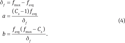
However, these definitions can lead to negative f′ values for individuals that are far below favg when favg is close to fmax. To prevent this situation, if

then a and b are defined as

A certain relationship between the maximum fitness of the population and the average fitness of the population is maintained with the following constraint equations:

where  is the scaled maximum fitness, favg is the average fitness of the population, and Cs is a scaling constant that specifies the number of expected copies of the best individual in the next generation. Additional best fitness individuals allowed in the population causes an increase in selection pressure, which causes faster convergence. This can lead to a premature convergence on the local optima.
4.3 Uniqueness Preservation
When uniqueness preservation is used, the algorithm disallows the generation of new individuals that are identical to any individual in the existing population. If an individual is generated that has a clone in the population, it is mutated until it is unique. The purpose of this mechanism is to maintain diversity in a population. This scheme comes with a small limitation: the search space must be smaller than the population size plus the number of children generated per generation.
It is possible for fitness scaling and uniqueness preservation to work in tandem, but in this work, uniqueness preservation is not used in the same run as fitness scaling. Instead, each method is used separately to compare their results.
4.4 Parallelization
GAs are inherently parallel processes that are typically performed serially. A GA is initialized by either generating a population of independently randomly generated individuals or by simply loading a seed population. Every generation, the genetic operators are performed on the population based on a static state. Fitness scaling occurs once before parent selection. The selection of pairs of parents and the subsequent creation of offspring via crossover and mutation could also be performed simultaneously, as each set of operations does not influence any other. The evaluation of each individual, at both initialization of the population and the generation of offspring, is an independent operation. This is important because fitness evaluation is typically the most computationally expensive portion of GA. Despite the structure of GAs, they are often designed to run as serial algorithms. However, on a machine with multiple processors, this inherent parallelism can be exploited for faster run times. The implementation of parallelization for the GA developed for this article is realized using the synchronous master–slave architecture of Grefenstette [5], in which a single master process performs all the evolutionary operations and multiple concurrent processes perform fitness function evaluations. With this design, given a machine with N processors, N concurrent fitness evaluation processes are possible. The machines used for the experiments had eight core processors and so could take advantage of up to eight concurrent fitness evaluation processes.
Experiments that required the comparison of statistical analysis of results therefore had 30 runs of each parameter set, each with a different random seed. The way this was accomplished was also in parallel. A shell script runs from a master machine to connect to 40 slave machines and on each of them starts a run of the GA. In the experiments, 40 machines are used instead of 30 because as many as 40 were available at a time, and this allowed as many as 10 runs to fail due to network interruption. Each machine saves a log file and a state file to a shared network drive. The log file format lists first the parameters used to run the GA and follows with four columns: the generation number, the best fitness in the current population, the average fitness in the population, and the best fitness found during the entire run of the GA. The reason to track the best found ever is that in any configuration that uses generational replacement of the population, it is possible to lose the best individual found and replace it with a less fit offspring.
The state file lists the integer representation of each member of the population at the end of each generation. Due to the large population sizes and the large number of concurrent experiments being run, only the most recent generation is recorded, with the previously written one being overwritten.
In case that a GA does not complete its run, a GA can be started with a state file as input to initialize the population. If the other parameters are the same, the course of the GA will continue as if it had not been interrupted. This allows the machines to be used by other processes, only running the GA during low-usage times.
4.5 Parameters
Every GA is subject to a set of parameters that control the specifics of each of its operators. These can be numerical settings or rates, such as population size, number of children to create per generation, and mutation rate, or they can be alternative definitions of operators, such as parent selection, recombination, mutation, survivor selection, or termination condition.
The GA used in this article uses the same operators for parent selection, recombination, and mutation as the described SGA. However, it differs in survival selection. Instead of generational survival selection, elitist survival selection is used, combining the child population with the current population, sorting by fitness and culling the worst, and leaving a constant population size. These operators are the same throughout this investigation. However, in a few experiments, the effects of different values for some of the numerical parameters, such as mutation rate and population size, are compared.
4.6 Implementation
The GA was implemented in C++ and compiled with the GNU C/C++ compiler (www.gnu.org). Each instance of the GA was executed on an 8 Intel® Xeon® W3520 (www.intel.com)at a 2.67-GHz core machine with 4 GB of RAM and 119.7 GB of hard disk space running the 64-bit version of GNU/Linux OS distribution Fedora 13 (www.fedoraproject.org)(Kernel Linux 2.6.34.7-61.fc13.x86 64). Each instance of the algorithm required a transmit code length, PSK constellation size, random seed, maximum number of concurrent threads, and the following GA parameters: number of generations, population size, children per generation, mutation rate, and flags to enable fitness scaling or uniqueness. Optionally, a text file can be used to seed the GA. If no seed file is provided, the initial population is uniformly randomly generated. Seeding has been shown effective [8] in GA approaches.
The output of the GA is two text files. One text file is a record of the algorithm’s progress, saving at the end of each generation three data: the population’s average MSE, the best MSE currently in the population, and the best MSE encountered so far. The other file is a save state, which contains the chromosomes of each individual in the current population. This can be used as an input file to seed or continue another execution of the algorithm.
5 Experiments and Results
A series of experiments were conducted, with 30 runs each and using a different random seed for each run. Each experiment seeks a different transmit code, increasing with length and PSK constellation size. The performance of the GA is compared against the parallelized version of the greedy MIA and a random transmit code generator. Each run of the greedy MIA is started with a uniformly randomly generated seed code instead of a zero vector. The random search generates the same number of codes as the GA, and reports the best code found. The number of codes evaluated during run of the GA depends on the number of offspring per generation and how many generations it runs. Although the GA may potentially find multiple good solutions during a single run, only the best transmit code per run is used in this analysis.
In this section, the experimental results are presented and the effectiveness of the GA is discussed. With different values for parameters such as population size, children per generation, and mutation rate, to name a few, a GA will perform differently. Clearly, finding an optimal configuration for a given problem is at least as difficult as solving the problem to begin with. Such meta-optimization is not approached in this article.
However, there are versions of the GA that use fitness scaling or uniqueness to preserve diversity. In some experiments, their effectiveness is compared against a GA without any such operator. The results of each experiment are summarized in tables that list the mean MSE, best MSE, worst MSE, and standard deviation (SD) of the set of transmit codes each algorithm found. Box plots are also used to depict the results.
Series of statistical tests are conducted after each experiment. First, one-way analysis of variance (ANOVA) is used to determine if there is a significant difference in the means of results. Because each experiment compares more than two algorithms, it is not known which means are significantly different from each other. Therefore, if a difference is found, Tukey honestly significant difference (HSD) [1] is used to make multiple comparisons. The results of the Tukey HSD tests are summarized by classifying the results of the algorithms into groups that are not significantly different. Finally, pairwise Wilcoxon rank sum tests [13] are performed to test whether the distributions of the results differ. For the Wilcoxon rank sum tests, p-values are adjusted using the Bonferroni correction method [12].
5.1 Length 13 2 PSK
The first experiment conducted seeks a length 13, binary (2 PSK) transmit code. The longest known Barker code is of length 13; thus, in this case, the global minimum is known and an exhaustive search would only take 213 (8192) evaluations. The GA has a population size of 100, has 100 children per generation, and terminates after 20 generations or 20,000 evaluations. Each algorithm is run 30 times, and the results are summarized in Table 1 and Figure 1.
Length 13 2 PSK Results.
| Algorithm | Mean | Best | Worst | Success Rate |
|---|---|---|---|---|
| GA | 0.1533 | 0.0718 | 0.2270 | 0.1667 |
| MIA | 0.2926 | 0.1558 | 0.4143 | 0 |
| RAND | 0.0964 | 0.0718 | 0.1558 | 0.7000 |

Length 13 2 PSK Box Plot Results.
The ANOVA reveals that there is a statistically significant difference somewhere in the mean result of the algorithms. Tukey HSD test results are used to classify the algorithms, and each one has a significantly different mean, as illustrated in Table 2. Finally, the Wilcoxon pairwise rank sum test further demonstrates that the distributions in the three groups differ significantly from each other.
Length 13 2 PSK: Tukey HSD Class Memberships.
| Algorithm | Class Memberships |
|---|---|
| PMIA | a |
| GA | b |
| RAND | c |
5.2 Length 52 2 PSK
This experiment seeks another binary transmit code, this time with length 52. An exhaustive search would take 252 (~4.5e + 15) evaluations. The GA has a population size of 500, has 500 children per generation, and terminates after 200 generations or 100,000 evaluations. Each algorithm is run 30 times, and the results are summarized in Table 3 and Figure 2.
Length 52 2 PSK Results.
| Algorithm | Mean | Best | Worst | SD |
|---|---|---|---|---|
| GA | 0.2632 | 0.2134 | 0.3316 | 0.02897 |
| MIA | 0.2738 | 0.2231 | 0.3924 | 0.04207 |
| RAND | 0.3163 | 0.2408 | 0.3479 | 0.02315 |

Length 52 2 PSK Box Plot Results.
The ANOVA reveals that there is a statistically significant difference somewhere in the mean result of the algorithms. However, both Tukey multiple comparisons of means (Table 4) and the pairwise Wilcoxon rank sum tests show that difference exists between the random search and the greedy MIA or the GA. There is no significant difference in the mean or distribution of the results of the greedy MIA or the GA.
Length 52 2 PSK: Tukey HSD Class Memberships.
| Algorithm | Class Memberships |
|---|---|
| MIA | a |
| GA | a |
| RAND | b |
5.3 Length 58 2 PSK
This experiment seeks another binary transmit code, this time with length 58. An exhaustive search would take 258 (~2.8e + 17) evaluations. The GA has a population size of 500, has 500 children per generation, and terminates after 200 generations or 100,000 evaluations. In this experiment, different modifications of the GA are tried. A standard GA, a GA using fitness scaling, and a GA using uniqueness preservation are all compared. In addition, each variation of the GA is also run with two different mutation rates. A mutation rate of 0.03 mutations per 1000 chips transferred is compared against a mutation rate of 0.17 mutations per 1000 chips. Each algorithm is run 30 times, and the results are summarized in Table 5 and Figure 3.
Length 58 2 PSK Results.
| Algorithm | Mean | Best | Worst | SD |
|---|---|---|---|---|
| GA-lu | 0.2069245 | 0.165078 | 0.2261300 | 0.01281314 |
| GA-mu | 0.2079898 | 0.178671 | 0.2317660 | 0.01425155 |
| GA-mf | 0.2625325 | 0.201165 | 0.3086400 | 0.02761104 |
| GA-m | 0.2635027 | 0.215362 | 0.3193720 | 0.03009706 |
| GA-l | 0.2752430 | 0.175345 | 0.3358340 | 0.03435993 |
| GA-lf | 0.2808252 | 0.201273 | 0.3414180 | 0.03227592 |
| MIA | 0.2882690 | 0.208831 | 0.3887021 | 0.04464315 |
| RAND | 0.3268788 | 0.277506 | 0.3563460 | 0.01996862 |

Length 58 2 PSK Box Plot Results.
ANOVA reveals that there is a statistically significant difference in the mean result of the algorithms. Tukey HSD test results are used to classify the algorithms (Table 6). Both of the GAs that used uniqueness preservation are classified as having a significantly different mean from the rest of the algorithms. The GAs that used the higher mutation rate outclassed the GAs with the lower mutation rate and no uniqueness preservation, which did not have a significantly different mean from the greedy MIA. Finally, the Wilcoxon pairwise rank sum test further demonstrates the statistical relationships between the distributions of each set of results.
Length 58 2 PSK: Tukey HSD Class Memberships.
| Algorithm | Class Memberships |
|---|---|
| Gals | ab |
| GAlu | c |
| GAmf | a |
| GAms | a |
| GAmu | c |
| MIA | b |
| RAND | d |
| GAlf | ab |
5.4 Length 51 32 PSK
In this experiment, polyphasic codes of length 51 and 32 PSK are generated. An exhaustive search would take 3251 (~5.7e + 76) evaluations. The GA has a population size of 500, has 500 children per generation, and terminates after 300 generations or 150,000 evaluations. In this experiment, different modifications of the GA are tried. A standard GA, a GA using fitness scaling, and a GA using uniqueness preservation are all compared. A mutation rate of 0.19 mutations per 1000 chips transferred is used throughout the experiment. Each algorithm is run 30 times, and the results are summarized in Table 7 and Figure 4.
Length 51 32 PSK Results.
| Algorithm | Mean | Best | Worst | SD |
|---|---|---|---|---|
| GAf | 0.1754435 | 0.141882 | 0.2082470 | 0.01692452 |
| GAs | 0.1744988 | 0.141882 | 0.2082470 | 0.01648276 |
| GAu | 0.1077868 | 0.081401 | 0.1381190 | 0.01251883 |
| MIA | 0.0878632 | 0.062018 | 0.1103647 | 0.01272620 |
| RAND | 0.3268788 | 0.277506 | 0.4548510 | 0.01568197 |

Length 51 32 PSK Box Plot Results.
ANOVA reveals that there is a statistically significant difference in the mean result of the algorithms. Tukey HSD test results are used to classify the algorithms. The standard GA and the GA using fitness scaling were classified as having insignificantly different means from each other but significantly different from the rest (Table 8). The greedy MIA mean MSE is better by >1 SD than the next closest algorithm, the GA using uniqueness preservation. The Wilcoxon pairwise rank sum test demonstrates that the distributions in the three groups differ significantly from each other.
Length 51 32 PSK: Tukey HSD Class Memberships.
| Algorithm | Class Memberships |
|---|---|
| GAs | a |
| GAu | b |
| MIA | c |
| RAND | d |
| GAf | a |
5.5 Length 17 64 PSK
In this experiment, polyphasic codes of length 17 and 64 PSK are generated. An exhaustive search would take 6417 (~5.0e + 30) evaluations. The GA varies in population size in this experiment. One set of GAs has a population size of 500, has 500 offspring per generation, and terminates after 3000 generations or 1,500,000 evaluations. The other set of GAs has a population size of 5000, has 5000 offspring per generation, and terminates after 600 generations or 3,000,000 evaluations.
In this experiment, different modifications of the GA are tried. A standard GA, a GA using fitness scaling, and a GA using uniqueness preservation are all compared. A mutation rate of 0.19 mutations per 1000 chips transferred is used throughout the experiment. Each algorithm is run 30 times, and the results are summarized in Table 9 and Figure 5.
Length 17 64 PSK Results.
| Algorithm | Mean | Best | Worst | SD |
|---|---|---|---|---|
| GAfl | 0.09090319 | 0.04486430 | 0.1498160 | 0.02600308 |
| GAfs | 0.08726232 | 0.04192010 | 0.1402750 | 0.02263069 |
| GAl | 0.09181526 | 0.05430950 | 0.1231710 | 0.01892948 |
| GAs | 0.10200423 | 0.04623240 | 0.1788180 | 0.02808770 |
| GAul | 0.08491796 | 0.04225520 | 0.1161510 | 0.01833392 |
| GAus | 0.08069726 | 0.04356430 | 0.1410860 | 0.02888958 |
| MIA | 0.09834705 | 0.05479663 | 0.1463733 | 0.02227150 |
| Rand | 0.22806287 | 0.19250400 | 0.2535850 | 0.01580852 |

Length 17 64 PSK Box Plot Results.
ANOVA confirms that there is a statistically significant difference in the mean result of the algorithms, as illustrated in Table 24. The differences given by Tukey HSD multiple comparisons of means are calculated, and the resulting classifications are shown in Table 10.
Length 17 64 PSK: Tukey HSD Class Memberships.
| Algorithm | Class Memberships |
|---|---|
| GAfs | ab |
| GAl | ab |
| GAs | a |
| GAul | ab |
| GAus | b |
| MIA | ab |
| RAND | c |
| GAfl | ab |
5.6 Length 49 64 PSK
In this experiment, polyphasic codes of length 49 64 PSK are generated. An exhaustive search would take 6449 (~3.1e + 88) evaluations. The GA has a population size of 1000, has 1000 offspring per generation, and terminates after 500 generations or 500,000 evaluations. In this experiment, different modifications of the GA are tried. A standard GA, a GA using fitness scaling, and a GA using uniqueness preservation are all compared. A mutation rate of 0.20 mutations per 1000 chips transferred is used throughout the experiment. The data from the random search algorithm are missing due to an error at run time that has not been corrected at the time of writing. Each algorithm is run 30 times, and the results are summarized in Table 11 and Figure 6.
Length 49 64 PSK Results.
| Algorithm | Mean | Best | Worst | SD |
|---|---|---|---|---|
| GAf | 0.13069591 | 0.09612920 | 0.1756330 | 0.018230771 |
| GA | 0.12467841 | 0.09612920 | 0.1639320 | 0.016499612 |
| GAu | 0.09467253 | 0.07622120 | 0.1152980 | 0.009212712 |
| MIA | 0.08192220 | 0.04752182 | 0.1032973 | 0.012021836 |

Length 49 64 PSK Box Plot Results.
ANOVA confirms that there is a statistically significant difference in the mean result of the algorithms. The resulting classifications given by Tukey HSD are shown in Table 12. The results of the pairwise comparisons using the Wilcoxon rank sum test support these classifications.
Length 49 64 PSK: Tukey HSD Class Memberships.
| Algorithm | Class Memberships |
|---|---|
| GAs | a |
| GAu | b |
| MIA | c |
| GAf | a |
6 Conclusion
This article presented an SGA that attempts to find transmit codes with minimal radar target profile expected error. The results of the GA versions using fitness scaling and uniqueness preservation were compared with an existing greedy search method.
When searching for binary codes, the GA-generated results as good as or better than the greedy method. However, when searching for polyphase codes, the GA had equal or inferior results to the greedy method. In the case of length 51 32 PSK code, the greedy algorithm-generated codes with mean MSE better by >1 SD than the closest GA. In the case of length 17 64 PSK code, some versions of the GA had the same performance as the greedy method. In the largest search space, length 49 64 PSK, the greedy MIA found the best codes and was significantly better than the codes the GAs found.
GAs with varying mutation rates and population sizes were compared. Two different mutation rates were used when searching for length 58 2 PSK codes and did not cause statistically different results. Two different population sizes were used when searching for length 17 64 PSK codes and did not cause statistically different results.
Two diversity-preserving measures, fitness scaling and uniqueness preservation, were used in several of the experiments, as well as the standard GA without any such measure. In all the cases in which these two methods were compared (length 58 2 PSK, length 51 32 PSK, length 17 64 PSK, length 49 64 PSK), the GAs using fitness scaling found slightly better results but did not find statistically significantly different results than the standard GA. The GA using uniqueness preservation found statistically significantly better results than both the standard GA and the GA using fitness scaling.
In terms of future work, although the GA did well in finding good binary radar transmit codes, when searching for longer codes with larger constellations, the GA did not perform as well as the greedy MIA. Both algorithms used the same heuristic, but the GA required many more evaluations to find good solutions, whereas the greedy algorithm quickly converged.
However, the GA could certainly be improved. One way to cut down on the number of evaluations the GA requires would be to keep a table of the fitness of previously found individuals. It is possible to regenerate and reevaluate a previously found solution. This wastes computation time. Before implementing such a mechanism, it would be prudent to run first an experiment that keeps a count of every unique individual code generated during the course of GA. If, for a given problem set, a good portion of the evaluations is for previously generated individuals, then this would be a wise optimization.
The fact that GAs using uniqueness preservation performed significantly better than any other GA configuration suggests that the more standard features of the GA are not well suited for this problem. Only a few experiments were conducted to compare certain parameters of the GA such as mutation rate and population size. Any future investigation would require some tuning of these parameters. Variations in parent selection and survival selection methods should also be explored. The elitist survival selection method used in this project may be too aggressive and have causes a premature convergence of the population, even with fitness selection and uniqueness preservation in place. The same could be said of the fitness proportional parent selection.
Mutation rates, which were kept relatively low throughout this investigation, may need to be raised as the search space increases. Alternatively, instead of keeping a fixed mutation rate for every gene in all the individuals in the population, a technique from evolutionary strategies could be used, which, along with the solutions, keeps a vector of mutation rates for each individual, and these mutation rate data are evolved along with the solutions [6].
Another diversity preservation method called crowding could be investigated as well. Crowding is similar to uniqueness preservation, but instead of disallowing the generation of new individuals that are identical to any individual in the existing population, it replaces the most similar member of the population [9].
Although the parallelization scheme used in this project took advantage of all the processing power available on a single multi-core machine, a networked approach with remote machines performing fitness evaluations at less than full capacity would be much better suited to today’s cloud-based computing, as powerful networked computers become ubiquitous.
Another approach could be to modify the GA to run in phases. First, generate codes with a smaller constellation early in the run; then, when the population has converged, increase the constellation size, translate the population’s codes to the new size, and dramatically increase the mutation rate for a few generations. This approach can be repeated until the desired constellation size is reached and the population converges. This scheme could be implemented using the GA developed for this project and a function that translates transmit codes from one constellation size to another. Each phase would represent a single run of the GA. The translation function would transform the state file produced, and the next phase of the GA would be another run seeded with the transformed state file. Finally, another scheme that would seed the GA would be a hybrid approach that would generate the initial population of the GA using multiple runs of the greedy marginal improvement algorithm. This hybrid approach would require a GA that is improved using any of the methods suggested in this article.
Bibliography
[1] H. Abdi and L. J. Williams, Tukey’s honestly significant difference (HSD) test, in: Encyclopaedia of Research Design, N. Salkind, ed., Sage, Thousand Oaks, CA, 2010.Search in Google Scholar
[2] B. Boudamouz, P. Millot and C. Pichot, MIMO antenna design with genetic algorithm for TTW radar imaging, in: Proceedings of the 9th European Radar Conference (EuRAD), pp. 150–153, 2012.Search in Google Scholar
[3] G. Fan and W. Deng, MIMO radar transmit beam pattern synthesis based on genetic algorithm, in: Proceedings of the 5th Global Symposium on Millimeter Waves (GSMM 2012), pp. 445–448, Harbin, China, 2012.10.1109/GSMM.2012.6314094Search in Google Scholar
[4] D. E. Goldberg, Genetic algorithms in search, optimization and machine learning, 2nd ed., Addison-Wesley Longman Publishing Co., Boston, MA, 1989.Search in Google Scholar
[5] J. J. Grefenstette, Parallel adaptive algorithms for function optimization, Technical Report No. CS-81-19, Computer Science Department, Vanderbilt University, Nashville, TN, 1981.Search in Google Scholar
[6] J. H. Holland, Adaptation in natural and artificial systems, University of Michigan Press, Ann Arbor, MI, 1975.Search in Google Scholar
[7] J. D. Jenshak, A fast method for generating transmit codes for radar, in: Proceedings of the Radar Conference, pp. 1–6, Rome, Italy, 2008.10.1109/RADAR.2008.4720804Search in Google Scholar
[8] B. A. Julstrom, Seeding the population: improved performance in a genetic algorithm for the rectilinear Steiner problem, in: Proceedings of the ACM Symposium on Applied Computing(SAC 94), pp. 222–226, 1994.10.1145/326619.326728Search in Google Scholar
[9] O. J. Mengshoel and D. E. Goldberg, The crowding approach to niching in genetic algorithms, Evol. Comput.16 (2008), 315–354.10.1162/evco.2008.16.3.315Search in Google Scholar PubMed
[10] L. Pengzheng, H. Xiaotao, W. Jian and M. Xile, Sensor placement of multistatic radar system by using genetic algorithm, in: Proceedings of the IEEE International Geoscience and Remote Sensing Symposium (IGARSS), pp. 4782–4785, 2012.Search in Google Scholar
[11] P. Wei, P. W. Li and Y. Jinsong, Adaptive genetic algorithm evidence model and its application for discriminating enemy radar operation intention, in: Proceedings of the 24th Chinese Control and Decision Conference (CCDC), pp. 1088–1093, 2012.Search in Google Scholar
[12] Wikipedia, 2013. Available at: en.wikipedia.org/wiki/Bonferroni_correction. Accessed May 2013.Search in Google Scholar
[13] C. J. Wild and G. A. F. Seber, Chance encounters: a first course in data analysis, Wiley, New York, 2000.Search in Google Scholar
[14] Z. Zhang, Y. Zhao and J. Huang, Array optimization for MIMO radar by genetic algorithms, in: Proceedings of the 2nd International Congress on Image and Signal Processing (CISP 09), pp. 1–4, 2009.10.1109/CISP.2009.5304413Search in Google Scholar
[15] M. Zomorrodi, Improved genetic algorithm approach for phased array radar design, in: Proceedings of the Asia-Pacific Microwave Conference (APMC), pp. 1850–1853, 2011.Search in Google Scholar
©2013 by Walter de Gruyter Berlin Boston
This article is distributed under the terms of the Creative Commons Attribution Non-Commercial License, which permits unrestricted non-commercial use, distribution, and reproduction in any medium, provided the original work is properly cited.
Articles in the same Issue
- Masthead
- Masthead
- Passing an Enhanced Turing Test – Interacting with Lifelike Computer Representations of Specific Individuals
- Automatically Detecting the Number of Logs on a Timber Truck
- Request–Response Distributed Power Management in Cloud Data Centers
- A Fast and Reliable Corner Detector for Non-Uniform Illumination Mineshaft Images
- Finding the Trustworthiness Nodes from Signed Social Networks
- Particle Swarm Optimization Neural Network for Flow Prediction in Vegetative Channel
- A Genetic Algorithm for Generating Radar Transmit Codes to Minimize the Target Profile Estimation Error