Individualized treatment rules under stochastic treatment cost constraints

4.1 Pathwise differentiability of the ATE

We first present a result regarding the pathwise differentiability of the ATE. Pathwise differentiability of the parameter of interest serves as the foundation for constructing asymptotically efficient estimators of this parameter, based on which an inferential procedure may be developed. Additional technical conditions are required and are provided in Section S1 in the Supplementary Material. For a distribution P ∈ ℳ , a function μ C : { 0 , 1 } × W → R , an ITR ρ , and a decision threshold τ ∈ R , we define pointwise the following functions:

One key condition we rely on is the following nonexceptional law assumption.

Under this condition, the true optimal ITR ρ 0 is identical to an indicator function. If all covariates are discrete, then we can plug in the empirical estimates into the identification formulae in Theorems 1 and 2 and show that the resulting estimators of the ATE are asymptotically normal by the delta method even when Condition B1 does not hold. We do not further pursue this simple case in this article, and thus need to rely on the nonexceptional law assumption, namely Condition B1, to account for continuous covariates. We list additional technical conditions in Supplement S1.

We can now provide a formal result describing the pathwise differentiability of the ATE parameter.

We note that the pathwise differentiability of P ↦ Ψ ρ P ℛ ( P ) was established in Theorem 3 in the study by Qiu et al. [9] for ℛ ∈ { FR , TP } . The other results can be proven using similar techniques. We presented the proof of these results in Supplement S4.2. In view of Theorem 3, it follows that the ATE parameter Ψ ℛ is pathwise differentiable at P 0 with nonparametric canonical gradient:

for ℛ ∈ { FR , RD , TP } .

4.2 Proposed estimator and asymptotic linearity

We next present our proposed nonparametric procedure for estimating an optimal ITR ρ 0 and the corresponding ATE ψ 0 . We will generally use subscript n to denote an estimator with sample size n and add a hat to a nuisance function estimator that is targeted toward estimating ϕ 0 .

1. Use the empirical distribution P ˆ W , n of W as an estimate of the true marginal distribution of W . Compute estimates μ n Y , μ n C , μ n T , δ n Y and δ n C of μ 0 Y , μ 0 C , μ 0 T , δ 0 Y and δ 0 C , using flexible regression methods. Recall that μ 0 Y ( t , w ) = E 0 [ Y ∣ T = t , W = w ] , μ 0 C ( t , w ) = E 0 [ C ∣ T = t , W = w ] , δ 0 Y ( v ) = E 0 [ μ 0 Y ( 1 , W ) − μ 0 Y ( 0 , W ) ∣ V = v ] , and δ 0 C ( v ) = E 0 [ μ 0 C ( 1 , W ) − μ 0 C ( 0 , W ) ∣ V = v ] . Define pointwise Δ n C ( w ) ≔ μ n C ( 1 , w ) − μ n C ( 0 , w ) .

2. Estimate an optimal ITR:

   1. Estimate ϕ 0 = E 0 [ μ 0 C ( 0 , W ) ] with a one-step correction estimator:

      ϕ n ≔ 1 n ∑ i = 1 n μ n C ( 0 , W i ) + ( 1 − T i ) ( C i − μ n C ( 0 , W i ) ) 1 − μ n T ( W i ) .

   2. Let ξ n ≔ δ n Y / δ n C , Γ n : τ ↦ 1 n ∑ i : ξ n ( V i ) > τ Δ n C ( W i ) and γ n : τ ↦ 1 n ∑ i : ξ n ( V i ) = τ Δ n C ( W i ) . For any k ∈ [ 0 , ∞ ] , define η n ( k ) ≔ inf { τ : Γ n ( τ ) ≤ k − α ϕ n } , τ n ( k ) ≔ max { η n ( k ) , 0 } and

      d n , k : v ↦ k − α ϕ n − Γ n ( η n ( k ) ) γ n ( η n ( k ) ) : if ξ n ( v ) = η n ( k ) and γ n ( η n ( k ) ) > 0 , I { ξ n ( v ) > η n ( k ) } : otherwise.

      The rule d n , k is the sample analog of an ITR that prescribes treatment to those with the highest values of ξ 0 ( V ) , regardless of whether the treatment is harmful, until treatment resources run out.

   3. Compute k n , which is used to define an estimate of ρ 0 for which the plug-in estimator is asymptotically linear under conditions, as follows:

      1. if τ n ( κ ) > 0 and there is a solution in k ∈ [ 0 , ∞ ) to

         (5) 1 n ∑ i = 1 n d n , k ( V i ) Δ n C ( W i ) + C i − μ n C ( T i , W i ) t i + μ n T ( W i ) − 1 + α ϕ n = κ ,

         then take k n to be this solution;

      2. otherwise, set k n = κ .

   4. Estimate ρ 0 using the sample analog of ρ 0 with treatment resource constraint k n , namely,

      ρ n : v ↦ k n − α ϕ n − Γ n ( τ n ( k n ) ) γ n ( τ n ( k n ) ) : if ξ n ( v ) = τ n ( k n ) and γ n ( τ n ( k n ) ) > 0 I { ξ n ( v ) > τ n ( k n ) } : otherwise.

3. Obtain an estimate ρ n ℛ of the reference ITR ρ 0 ℛ as follows:

   1. For ℛ = FR , take ρ n ℛ to be ρ FR .

   2. For ℛ = RD ,

      1. obtain a targeted estimate μ ˆ n C ( 1 , ⋅ ) of μ 0 C ( 1 , ⋅ ) : run an ordinary least-square linear regression with outcome C , covariate 1 / ( T + μ n T ( W ) − 1 ) , offset μ n C ( T , W ) , and no intercept. Take μ ˆ n C to be the fitted mean model;

      2. take ρ n ℛ to be the constant function w ↦ min 1 , ( κ − ϕ n ) / 1 n ∑ i = 1 n Δ ˆ n C ( W i ) , where we define pointwise Δ ˆ n C ( w ) ≔ μ ˆ n C ( 1 , w ) − μ ˆ n C ( 0 , w ) .

   3. For ℛ = TP , take ρ n ℛ to be μ n T .

4. Estimate ATE of ρ 0 relative to the reference ITR ρ 0 ℛ with a TMLE ψ n :

   1. obtain a targeted estimate μ ˆ n Y of μ 0 Y : run an ordinary least-square linear regression with outcome Y , covariate [ ρ n ( V ) − ρ n ℛ ( W ) ] / [ T + μ n T ( W ) − 1 ] , offset μ n Y ( T , W ) , and no intercept. Take μ ˆ n Y to be the fitted mean function.

   2. with P ˆ n being any distribution with components μ ˆ n Y and P ˆ W , n , take

      ψ n ≔ Ψ ρ n ( P ˆ n ) − Ψ ρ n ℛ ( P ˆ n ) = 1 n ∑ i = 1 n [ ρ n ( V i ) − ρ n , i ℛ ] [ μ ˆ n Y ( 1 , W i ) − μ ˆ n Y ( 1 , W i ) ] ,

      where ρ n , i ℛ is defined as ρ n ℛ ( W i ) or ρ n ℛ ( V i ) depending on the covariate used by the reference ITR.

The aforementioned procedure is similar to that proposed in the study by Qiu et al. [9]. One key difference is the use of the refined estimator k n of κ obtained via the estimating equation (5), which is a key to ensuring the asymptotic linearity of ψ n . Another difference is that the denominator of ξ n is now δ n C , which is consistent with our different definition of the unit value for solving the fractional knapsack problem (2). Similar to TMLE for other problems, when C or Y has known bounds (e.g., the closed interval [ 0 , 1 ] ), to obtain a corresponding targeted estimate that respect the known bounds, we may use logistic regression rather than ordinary least squares [36].

The aforementioned procedure has both similarities and substantial differences compared to the estimation procedure proposed by Sun et al. [11]. The main difference is that our procedure is targeted towards efficient estimation of and inference about the ATE of ψ 0 of the optimal ITR under a nonparametric model, while Sun et al. [11] focused on estimating the optimal ITR ρ 0 and does not evaluate this optimal ITR. This leads to a key difference between the two procedures when estimating the optimal ITR: we need to solve an estimating equation (5), which is crucial to ensuring that the estimator ψ n is asymptotically linear, while Sun et al. [11] do not. The requirement of solving (5) is related to the nature of the fractional knapsack problem discussed in Remark 3, and we conjecture that such a calibration on the resource used is necessary for general problems of the same nature. Our procedure is also related to the method in Sun [12]. Sun [12] relied on the availability of asymptotically normal estimators of both the average benefit and average resource used (Assumption 2.4), a nontrivial requirement when the propensity score μ 0 T is unknown in observational studies. Our procedure essentially produces such estimators: in Step 4, an asymptotically normal estimator of the ATE is constructed, whereas an asymptotically normal estimator of the expected resource is produced in Step 2 and used to calibrate the resource expenditure of the estimated optimal ITR ρ n in Step 2(c).

We now present results on the asymptotic linearity and efficiency of our proposed estimator. We state and discuss the technical conditions required by the theorem below in Supplement S1.

To conduct inference about ψ 0 , we can directly plug the estimators of nuisance functions into D ℛ ( P 0 ) to obtain a consistent estimator of D ℛ ( P 0 ) , and then take the sample variance to obtain a consistent estimator of the asymptotic variance σ 0 2 . The proof of Theorem 4 can be found in Supplements S4.3 and S4.4.

5.1 Simulation setting

In this simulation study, we investigate the performance of our proposed estimator of the ATE of an optimal ITR relative to specified reference ITRs. We focus here on the setting α = 1 . This scenario is more difficult than the case α = 0 because it requires the estimation of ϕ 0 .

We generate data from a model in which the treatment T is an IV and both the treatment cost C and outcome Y are binary. This data-generating mechanism satisfies all causal conditions and has an unobserved confounder between treatment cost and outcome. We first generate a trivariate covariate W = ( W 1 , W 2 , W 3 ) , where W 1 ∼ Unif ( − 1 , 1 ) , W 2 ∼ Bernoulli ( 0.8 ) , and W 3 ∼ N ( 0 , 1 ) are mutually independent. We also simulate an unobserved treatment-outcome confounder U ∼ Bernoulli ( 0.5 ) independently of W , and then simulate T , C , and Y as follows:

We introduce U in the data-generating mechanism to emphasize that we do not require assumptions on the joint distribution of treatment cost and outcome conditional on covariates. We consider all three reference ITRs ℛ ∈ { FR , RD , TP } , where we set ρ FR : v ↦ 0 . We set κ = 0.68 , which is an active constraint with τ 0 > 0 and ρ 0 RD < 1 .

The ITRs we consider are based on all covariates – that is, we take V ( W ) = W . We estimate the nuisance functions using the Super Learner [43] with library including a logistic regression, generalized additive model with logit link [44], gradient boosting machine [45,46, 47], support vector machine [48,49], and neural network [50,51]. Because none of the nuisance functions follows a logistic regression model, the resulting ensemble learner is not expected to achieve the parametric convergence rate. Since both C and Y are binary, we use logistic regression rather than ordinary least squares to obtain their corresponding targeted estimates in Section 4.2. We consider sample size n ∈ { 500 , 1,000 , 4,000 , 16,000 } and run 1000 Monte Carlo repetitions for each sample size. We implement the algorithm that incorporates cross-fitting discussed in Remark 6 and described in Section S3 in the Supplementary Material.

To evaluate the performance of our proposed estimator, we investigate the bias and root-mean-squared error (RMSE) of the estimator. We also investigate the coverage probability and the width of nominal 95% Wald CIs constructed using influence function-based standard error estimates. We further investigate the probability that our confidence lower limit falls below the true ATE, that is, the coverage probability of the 97.5% Wald confidence lower bound.

5.2 Simulation results

Table 1 presents the performance of our proposed estimator in this simulation. For sample sizes 500, 1,000 and 4,000, the CI coverage of our proposed method is lower than the nominal coverage 95%. When sample size is larger (16,000), the CI coverage of our proposed method increases to 90–93%. The coverage of the confidence lower bounds is much closer to nominal (97.5%) for all sample sizes considered, though, and is always approximately nominal when the sample size is large. For all reference ITRs, the bias and RMSE of our proposed estimator appear to converge to zero faster than and at the same rate as the square root of sample size, respectively. All biases are negative, which is expected in view of Remark 6. All standard errors underestimate the variation of the estimator with the extent decreasing as sample size increases.

Figure 1 presents the width of the Wald CIs scaled by the square root of sample size n . Our theory indicates that the CI width should shrink at a root- n rate, and our simulation results are consistent with this. There are some outlying cases of extremely wide or narrow CIs. This is expected for small sample sizes because the estimator of σ 0 2 in Theorem 4 resembles a sample mean and might not be close to σ 0 2 with high probability when the sample size is small. In practice, this issue might be slightly mitigated by fine-tuning the involved machine learning algorithms.

Figure 1

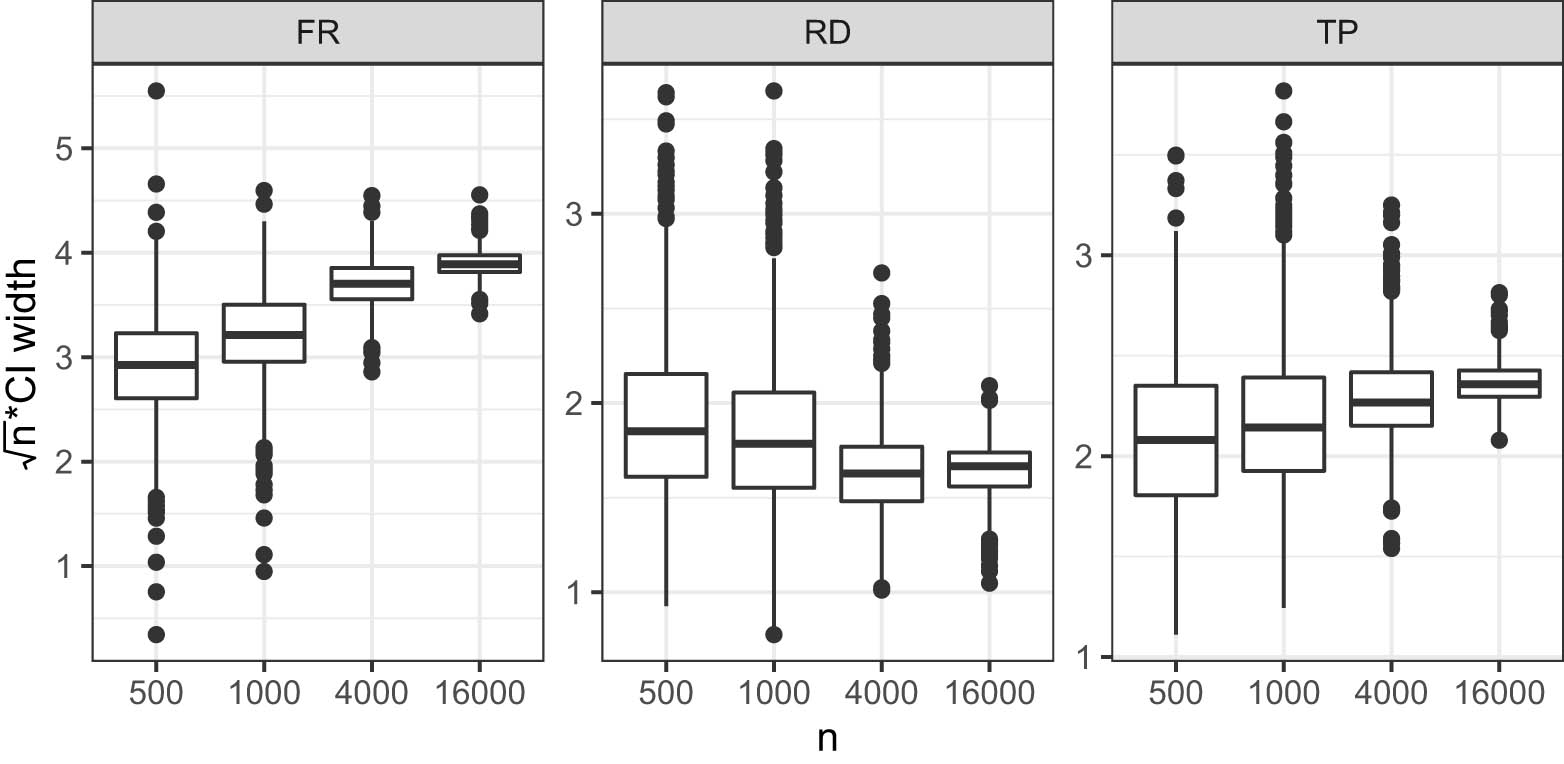
Boxplot of n × CI width for ATE relative to each reference IER.

As indicated in Theorem 4, theoretical guarantees for the validity of the Wald CIs rely on the nuisance function estimators converging to the truth sufficiently quickly. It appears that the undercoverage of our Wald CI in small samples may owe, in part, to poor estimation of these nuisance functions in small sample sizes. To illustrate how our procedure may perform with improved small-sample nuisance function estimators, we conducted another two simulations: one is identical to those reported earlier in all ways except that the nuisance function estimators μ n Y , μ n C , and μ n T are taken to be equal to the truth; the other is a simpler scenario under a lower dimension and a parametric model. The results are presented in Section S5 in the Supplementary material and suggest that our proposed estimator may achieve significantly better performance with improved machine learning estimators of the nuisance functions. This motivates seeking ways to optimize the finite-sample performance of the nuisance function estimators employed in future applications of the proposed method, possibly based on prior subject-matter expertise. The underestimation of standard errors in this simulation also motivates future work exploring whether there are standard error estimators with better finite-sample performance, for example, estimators based on the bootstrap.

References

[1] Rothwell PM. Subgroup analysis in randomised controlled trials: importance, indications, and interpretation. Lancet. 2005;365(9454):176–86. 10.1016/S0140-6736(05)17709-5Suche in Google Scholar PubMed
[2] Varadhan R, Segal JB, Boyd CM, Wu AW, Weiss CO. A framework for the analysis of heterogeneity of treatment effect in patient-centered outcomes research. J Clin Epidemiol. 2013;66(8):818–25. 10.1016/j.jclinepi.2013.02.009Suche in Google Scholar PubMed PubMed Central
[3] Chakraborty B, Moodie EEM. Statistical methods for dynamic treatment regimes. Statistics for biology and health. New York, NY: Springer; 2013. 10.1007/978-1-4614-7428-9Suche in Google Scholar
[4] Luedtke AR, van der Laan MJ. Statistical inference for the mean outcome under a possibly non-unique optimal treatment strategy. Annals Statistics. 2016;44(2):713–42. 10.1214/15-AOS1384Suche in Google Scholar PubMed PubMed Central
[5] Murphy SA. Optimal dynamic treatment regimes. J R Stat Soc B (Stat Methodol). 2003;65(2):331–55. 10.1111/1467-9868.00389Suche in Google Scholar
[6] Robins JM. Optimal structural nested models for optimal sequential decisions. New York, NY: Springer; 2004. p. 189–326. 10.1007/978-1-4419-9076-1_11Suche in Google Scholar
[7] Zhao Y, Zeng D, Rush AJ, Kosorok MR. Estimating individualized treatment rules using outcome weighted learning. J Am Stat Assoc. 2012;107(499):1106–18. 10.1080/01621459.2012.695674Suche in Google Scholar PubMed PubMed Central
[8] Luedtke AR, van der Laan MJ. Optimal individualized treatments in resource-limited settings. Int J Biostat. 2016;12(1):283–303. 10.1515/ijb-2015-0007Suche in Google Scholar PubMed PubMed Central
[9] Qiu H, Carone M, Sadikova E, Petukhova M, Kessler RC, Luedtke A. Optimal individualized decision rules using instrumental variable methods. J Am Stat Assoc. 2021;116(533):174–91. 10.1080/01621459.2020.1745814Suche in Google Scholar PubMed PubMed Central
[10] Qiu H, Carone M, Sadikova E, Petukhova M, Kessler RC, Luedtke A. Correction to: optimal individualized decision rules using instrumental variable methods. J Am Stat Assoc. 2021;(just-accepted):1–2. 10.1080/01621459.2020.1865166Suche in Google Scholar PubMed PubMed Central
[11] Sun H, Du S, Wager S. Treatment allocation under uncertain costs. 2021. arXiv: http://arXiv.org/abs/arXiv:210311066v1. Suche in Google Scholar
[12] Sun L. Empirical welfare maximization with constraints. 2021. arXiv: http://arXiv.org/abs/arXiv:210315298v1. Suche in Google Scholar
[13] Pfanzagl J. Estimation in semiparametric models. In: Estimation in semiparametric models. New York, NY, USA: Springer; 1990. p. 17–22. 10.1007/978-1-4612-3396-1_5Suche in Google Scholar
[14] van der Vaart AW. Asymptotic statistics. Cambridge, England: Cambridge University Press; 1998. 10.1017/CBO9780511802256Suche in Google Scholar
[15] van der Laan M, Rubin D. Targeted maximum likelihood learning. Int J Biostat. 2006;2(1):Article 11. doi: 10.2202/1557-4679.1043. 10.2202/1557-4679.1043Suche in Google Scholar
[16] van der Laan MJ, Rose S. Targeted learning in data science. New York, NY, USA: Springer; 2018. 10.1007/978-3-319-65304-4Suche in Google Scholar
[17] Neyman J. Sur les applications de la théorie des probabilités aux expériences agricoles: Essay des principles. (Excerpts reprinted and translated to English, 1990). Stat Sci. 1923;5:463–72. Suche in Google Scholar
[18] Rubin DB. Estimating causal effects of treatments in randomized and nonrandomized studies. J Educ Psychol. 1974;66(5):688–701. 10.1037/h0037350Suche in Google Scholar
[19] Butler EL, Laber EB, Davis SM, Kosorok MR. Incorporating patient preferences into estimation of optimal individualized treatment rules. Biometrics 2018;74(1):18–26. 10.1111/biom.12743Suche in Google Scholar PubMed PubMed Central
[20] Chen J, Fu H, He X, Kosorok MR, Liu Y. Estimating individualized treatment rules for ordinal treatments. Biometrics 2018;74(3):924–33. 10.1111/biom.12865Suche in Google Scholar PubMed PubMed Central
[21] Imai K, Li ML. Experimental evaluation of individualized treatment rules. J Am Stat Assoc. 2021;1–15. 10.1080/01621459.2021.1923511.Suche in Google Scholar
[22] Laber E, Zhao Y. Tree-based methods for individualized treatment regimes. Biometrika. 2015;102(3):501–14. 10.1093/biomet/asv028Suche in Google Scholar PubMed PubMed Central
[23] Lei H, Nahum-Shani I, Lynch K, Oslin D, Murphy SA. A “SMART” design for building individualized treatment sequences. Annual Rev Clin Psychol. 2012;8:21–48. 10.1146/annurev-clinpsy-032511-143152Suche in Google Scholar PubMed PubMed Central
[24] Petersen ML, Deeks SG, van der Laan MJ. Individualized treatment rules: Generating candidate clinical trials. Stat Med 2007;26(25):4578–601. 10.1002/sim.2888Suche in Google Scholar PubMed PubMed Central
[25] Qian M, Murphy SA. Performance guarantees for individualized treatment rules. Annal Stat. 2011;39(2):1180. 10.1214/10-AOS864Suche in Google Scholar PubMed PubMed Central
[26] Song R, Kosorok M, Zeng D, Zhao Y, Laber E, Yuan M. On sparse representation for optimal individualized treatment selection with penalized outcome weighted learning. Stat. 2015;4(1):59–68. 10.1002/sta4.78Suche in Google Scholar PubMed PubMed Central
[27] van der Laan MJ, Petersen ML. Causal effect models for realistic individualized treatment and intention to treat rules. Int J Biostat. 2007;3(1):Article 3. 10.2202/1557-4679.1022.Suche in Google Scholar PubMed PubMed Central
[28] Zhao YQ, Zeng D, Laber EB, Song R, Yuan M, Kosorok MR. Doubly robust learning for estimating individualized treatment with censored data. Biometrika. 2015;102(1):151–68. 10.1093/biomet/asu050Suche in Google Scholar PubMed PubMed Central
[29] Zhou X, Mayer-Hamblett N, Khan U, Kosorok MR. Residual weighted learning for estimating individualized treatment rules. J Am Stat Assoc. 2017;112(517):169–87. 10.1080/01621459.2015.1093947Suche in Google Scholar PubMed PubMed Central
[30] Abadie A. Semiparametric instrumental variable estimation of treatment response models. J Econom. 2003;113(2):231–63. 10.1016/S0304-4076(02)00201-4Suche in Google Scholar
[31] Imbens GW, Angrist JD. Identification and estimation of local average treatment effects. Econometrica. 1994;62(2):467–75. 10.2307/2951620Suche in Google Scholar
[32] Tchetgen Tchetgen EJ, Vansteelandt S. Alternative identification and inference for the effect of treatment on the treated with an instrumental variable. Harvard University Biostatistics Working Paper Series. 2013. Suche in Google Scholar
[33] Wang L, Tchetgen Tchetgen E. Bounded, efficient and multiply robust estimation of average treatment effects using instrumental variables. J R Stat Soc B (Stat Methodol). 2018;80(3):531–50. 10.1111/rssb.12262Suche in Google Scholar PubMed PubMed Central
[34] Robins J. A new approach to causal inference in mortality studies with a sustained exposure period-application to control of the healthy worker survivor effect. Math Modell. 1986;7(9–12):1393–512. 10.1016/0270-0255(86)90088-6Suche in Google Scholar
[35] Dantzig GB. Discrete-variable extremum problems. Operat Res. 1957;5(2):266–88. 10.1287/opre.5.2.266Suche in Google Scholar
[36] Gruber S, Van Der Laan MJ. A targeted maximum likelihood estimator of a causal effect on a bounded continuous outcome. Int J Biostat. 2010;6(1):Article 26. 10.2202/1557-4679.1260. Suche in Google Scholar PubMed PubMed Central
[37] van der Laan MJ, Luedtke AR. Targeted learning of the mean outcome under an optimal dynamic treatment rule. J Causal Inference. 2014;3(1):61–95.10.1515/jci-2013-0022Suche in Google Scholar PubMed PubMed Central
[38] Luedtke AR, van der Laan MJ. Super-learning of an optimal dynamic treatment rule. Int J Biostat. 2016;12(1):305–32. 10.1515/ijb-2015-0052Suche in Google Scholar PubMed PubMed Central
[39] Kennedy EH. Towards optimal doubly robust estimation of heterogeneous causal effects. 2020. arXiv: http://arXiv.org/abs/arXiv:200414497v3. Available from: http://arxiv.org/abs/2004.14497. Suche in Google Scholar
[40] Nie X, Wager S. Quasi-oracle estimation of heterogeneous treatment effects. Biometrika. 2021;108(2):299–319. 10.1093/biomet/asaa076Suche in Google Scholar
[41] Newey WK, Robins JR. Cross-fitting and fast remainder rates for semiparametric estimation. 2018. arXiv: http://arXiv.org/abs/arXiv:180109138v1. 10.1920/wp.cem.2017.4117Suche in Google Scholar
[42] Zheng W, van der Laan MJ. Cross-validated targeted minimum-loss-based estimation. New York, NY: Springer; 2011. p. 459–74. 10.1007/978-1-4419-9782-1_27Suche in Google Scholar
[43] van der Laan MJ, Polley EC, Hubbard AE. Super learner. Stat Appl Genetics Mol Biol. 2007;6(1):Article 25. 10.2202/1544-6115.1309. Suche in Google Scholar PubMed
[44] Hastie T, Tibshirani R. Generalized additive models. London: Chapman and Hall; 1990. Suche in Google Scholar
[45] Friedman JH. Greedy function approximation: a gradient boosting machine. Annal Stat. 2001;29(5):1189–232.10.1214/aos/1013203451Suche in Google Scholar
[46] Friedman JH. Stochastic gradient boosting. Comput Stat Data Anal. 2002;38(4):367–78. 10.1016/S0167-9473(01)00065-2Suche in Google Scholar
[47] Mason L, Baxter J, Bartlett PL, Frean M. Boosting algorithms as gradient descent; 2000. p. 512–8.Suche in Google Scholar
[48] Bennett KP, Campbell C. Support vector machines: hype or hallelujah? SIGKDD Explor Newsl. 2000;2(2):1–13. 10.1145/380995.380999Suche in Google Scholar
[49] Cortes C, Vapnik V. Support-vector networks. Machine Learning. 1995;20(3):273–97. 10.1007/BF00994018Suche in Google Scholar
[50] Bishop CM. Neural networks for pattern recognition. Oxford, England: Oxford University Press; 1995. 10.1093/oso/9780198538493.001.0001Suche in Google Scholar
[51] Ripley BD. Pattern recognition and neural networks. Cambridge, England: Cambridge University Press; 2014. Suche in Google Scholar
© 2022 the author(s), published by De Gruyter
This work is licensed under the Creative Commons Attribution 4.0 International License.
Artikel in diesem Heft
- Editorial
- Causation and decision: On Dawid’s “Decision theoretic foundation of statistical causality”
- Research Articles
- Simple yet sharp sensitivity analysis for unmeasured confounding
- Decomposition of the total effect for two mediators: A natural mediated interaction effect framework
- Causal inference with imperfect instrumental variables
- A unifying causal framework for analyzing dataset shift-stable learning algorithms
- The variance of causal effect estimators for binary v-structures
- Treatment effect optimisation in dynamic environments
- Optimal weighting for estimating generalized average treatment effects
- A note on efficient minimum cost adjustment sets in causal graphical models
- Estimating marginal treatment effects under unobserved group heterogeneity
- Properties of restricted randomization with implications for experimental design
- Clarifying causal mediation analysis: Effect identification via three assumptions and five potential outcomes
- A generalized double robust Bayesian model averaging approach to causal effect estimation with application to the study of osteoporotic fractures
- Sensitivity analysis for causal effects with generalized linear models