Estimating Average Treatment Effects Utilizing Fractional Imputation when Confounders are Subject to Missingness

1.1 Missing Data

Despite the best intentions of researchers, missing data is nearly impossible to avoid in real-world settings. Fortunately, as prevalent as missingness is, so too are methods with which to address missingness; however, the type of missingness matters when selecting a method.

Missing data occurs by way of one of three mechanisms in observational data. The first and simplest type is Missingness Completely at Random (MCAR) [6]. In this setting, whether or not an observation is missing is independent of both the observed and missing data. The second is Missingness at Random (MAR). Here, whether or not an observation is missing depends only on the observable data but not the missing data. Lastly, missing data can be Missing Not at Random (MNAR). In this setting, even after conditioning on all observed data, missingness will still depend on the missing portion of the data.

Confirming which missingness type is present for a given data set can not be validated from only the observed data. Little [7] proposed a chi-square based test capable of checking if the MCAR assumption was violated, and more recently Mohan and Pearl have been able to use m-graphs to refute instances where the MAR and MNAR assumptions were proposed but shown not to hold [8, 9]. Despite not being able to validate if a particular missingness model is true, it is still common for arguments towards one of these assumptions to be made, relying on the knowledge of subject matter experts for the data at hand. If the observed data is sufficient to explain the missingness, the MAR assumption is plausible, and it is this assumption we carry forward for the majority of our discussion. In Section 6 we will discuss the extension to MNAR.

1.2 Approaches to Address Missing Data

Many methods have been proposed to address missingness when assuming a MAR pattern. Two of the most common approaches in practice are complete case estimation (CC) and multiple imputation (MI). In particular, MI was favored by the National Research Council in 2010 as one of its preferred means of addressing missing data in clinical trials [10]. Under CC, all records with missing data are excluded, and treatment effects are estimated only on fully observed cases. CC can be biased under MAR; more importantly, if multiple variables have missing values, there will only be a small portion of complete cases in the data. By throwing out a large portion of the data, the effective sample size shrinks, inflating variances. Therefore, CC suffers from loss of efficiency by utilizing less of the observed data in the final analysis [11].

MI, on the other hand, is traditionally recommended for MAR in part due to its improved efficiency over CC and due to it being applicable to a wider range of missingness mechanisms. With MI, the full joint distribution of the data is estimated (either empirically or modeled based on distributional assumptions), and from this, a series of M new imputed data sets are drawn. In each imputed data set, MI fills in each missing value with an imputed value by sampling from the posterior predictive distribution of the missing value given the observed values. Then, full sample analyses can be applied to each imputed data sets, and these multiple results are summarized by an easy-to-implement combining rule for inference [12].

MI has produced valid frequentist inference in a wide range of applications [13]. At the same time, Rubin’s variance estimator for MI has been shown to not always be consistent [14, 15, 16, 17, 18, 19, 20, 21, 22]. For inference using MI consistent, imputation must be proper (see [12] for a precise definition). Practically speaking, for any proper imputations, under sufficiently regular models, Rubin’s combining rule provides a consistent estimator of the parameter of interest and a weekly unbiased estimator of its asymptotic variance. When the imputation model is correctly specified and the MAR assumption holds, Meng [23] showed that a sufficient condition for imputation to be proper is that the imputation model and the analysis model are congenial. For example, the imputation model is correctly specified and the analysis is efficient under the same model. Congeniality is sometimes more elusive than it would appear. Even when the imputation model is correctly specified, Yang and Kim [22] showed that MI is not necessarily congenial for method of moments estimation. Therefore, some common statistical procedures may be incompatible with MI. From a causal inference perspective, this poses a problem as the validity of Rubin’s variance estimator has not been fully explored for many full sample estimation methods used widely in causal inference. Certain otherwise unbiased and consistent full sample causal inference methods (outcome regression, weighting, matching, etc.) may lose these properties when applied in conjunction with MI and MI-produced data sets. Many of the most common estimates for average treatment effects are based on method of moments estimators and are thusly susceptible to inaccurate variance estimates when using Rubin’s variance estimator for MI. For researchers desiring to make causal claims when utilizing MI, it is imperative for the variance properties of their estimators to, therefore, be either validated or an alternative method must be proposed.

1.3 Fractional Imputation as an Alternative

As an alternative to CC and MI, there are likelihood-based methods that can be applied. When using these methods, the key insight is that under fully observed confounders, the full sample estimators are obtained by solving estimating equations. In the presence of partially observed confounders, the corresponding estimators can be obtained by solving conditional estimating equations which integrate out the missing confounders given the observed data. There are two difficulties in this approach. First, it requires consistent estimators in the conditional distribution of the missing confounders given the observed data, such as MLE. In the presence of missing values, an EM algorithm is typically used. Second, numerical integration is needed. Integration approximated by imputation was considered by many authors, such as Monte Carlo EM methods [24]. For Monte Carlo EM algorithms, in each E-step, the imputed values are regenerated, and thus the computation can be quite heavy. Also, the convergence of Monte Carlo sequence of the estimators is not guaranteed for fixed Monte Carlo sample size [25].

In practice, EM algorithms may not be feasible when the conditional expectation in the E-step is not available in a closed form. Instead, fractional imputation (FI) has been proposed to serve as a computational tool for implementing the expectation step (E-step) in the EM algorithm [24, 26, 27], which simplifies computation by drawing on importance sampling to obtain the fractional weights and reducing the iterative computation burden over other simulation methods such as Markov Chain Monte Carlo. See [28, 29, 30, 31] for applications of FI outside of the causal inference context. The main idea in FI is to produce a complete data set by imputation where each imputed value is associated with a fractional weight, by which the observed likelihood can be approximated by the weighted average of the imputed data likelihood. The resulting estimator approximates the maximum likelihood estimator.

For illustrative purposes, we can compare the format of the imputed data via FI to the more commonly encountered imputed data via MI. Suppose we have a data set where some of the records are subject to missingness. MI will attempt to address this missingness by creating M data sets where each imputed value is imputed exactly once in each of the M data sets as depicted in Figure 1. In this image X₁ is a fully observed covariate, and A and Y are fully observed treatment indicator and response variables respectively. X₂ is a covariate subject to missingness. R₁ and R₂ are missingness indicators for X₁ and X₂ where R_ij = 0 indicates X_j is missing for record i. Records with missingness are indicated in red on the left. The completed data sets (with X₂ imputed) are on the right with the records now including imputed values for X₂ highlighted in green.

Figure 1

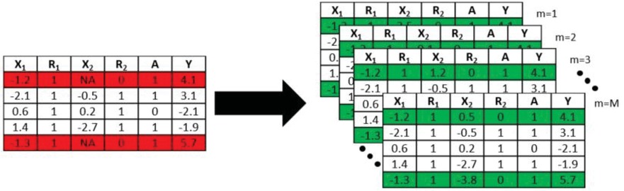
Imputed Data via MI

FI instead seeks to generate a single imputed data set, but one where each imputed record also includes a fractional weight. That fractional weight is indicative of how likely the imputed data is to occur under the distribution of the completed data set. Figure 2 shares all the same features as Figure 1 except now includes an additional column in the imputed data for the fractional weight (ω) that will be incorporated into analyses.

Figure 2

Imputed Data via FI

At its most basic level, the difference in imputation approach is analogous to a debate between a wide vs a tall data set. It could even be argued that when recombining data sets imputed via MI an implicit "weight" of 1/M is assigned to every record. This implicit 1/M weight acts similarly to the fractional weights ω generated via FI. The important distinction between MI and FI lies in how the final "weights" assigned to each imputed record are produced. The weight generation process for FI will be discussed in more depth in Section 3. For the time being, we will assume these weights are generated appropriately and can be incorporated easily into further analyses.

FI is sufficiently versatile that, like MI, it can be deployed along-side both continuous and categorical variables. Under the same common regularity conditions as seen often with MI, we show that the FI estimators are consistent and asymptotically normal. The remainder of this paper focuses on expanding FI into the causal literature by developing an FI-based method for estimating causal treatment effects. Once developed we will validate the method relative to existing causal inference methods. Specifically, we investigate the comparative performance of FI vs MI and CC for estimating causal treatment effects when confounders are subject to missingness.

In summary, the proposed FI framework achieves desirable properties for causal inference:

1. the same fractionally imputed data set allows for applying general full-sample estimators (which solve certain estimating equations) of the average treatment effect, including regression estimators, inverse probability of weighting estimators, and augmented weighting estimators;

2. the FI estimators are asymptotically linear and therefore allow resampling methods for variance estimation and inference, which is simple to implement in practice;

3. the unified FI inference has theoretical guarantees and offers a solution to the uncongeniality issue of MI;

4. and lastly, FI is not only statistically efficient but also computationally efficient compared to MI, as demonstrated via simulation and real-world application.

The rest of the article is organized as follows. We begin in Section 2 with a description of notation and assumptions. In Section 3 we fully outline the FI process as well as derive the resulting variance estimator for the treatment effect estimator. We implement a simulation study in Section 4 comparing the accuracy and precision of treatment effect estimators when the missingness is addressed by CC, MI, and FI. Section 5 provides a demonstration of FI’s utilization with a real-world health data set. Finally, in Section 6, we end with a discussion of the results and of the implication they have on current and future causal work.

2.1 Treatment Effect Estimation Notation

Following Neyman [32] and Rubin [33] we use the potential outcomes framework. Treatment is denoted by A_i ∈ {0, 1}, where 0 and 1 are labels for control and treatment respectively. For each subject i, define a pair of potential outcomes {Y_i(1), Y_i(0)} which represent the outcomes if the subject was treated, Y_i(1), and if he or she was not, Y_i(0). Implicit in this notation, we make the stable unit treatment value assumption [34]. The observed outcome for subject i is then Y_i = Y_i(A_i). Let X_i be the vector of confounders for subject i. We assume that {X_i , A_i, Y_i(1), Yi(0)}i=1nare independent draws from the distribution {X, A, Y(1), Y(0)}, and therefore, {(Xi,Ai,Yi)}i=1nare independent and identically distributed. The conditional treatment effect is τ(X) = E{Y(1) − Y(0) | X}, and the average treatment effect is τ₀ = E{τ(X)}. The average treatment effect cannot be estimated without further assumptions, because for each subject only one potential outcome is observed. The common assumptions for identifying the average treatment effect [1] are as follows:

Assumption 1 (Ignorability). Y(a)⊥A | X for a = 0,1, where ⊥ means "is conditionally independent of".

Assumption 2 (Sufficient overlap). With probability 1, 0 < c₁ ≤ e(X) ≤ c₂ < 1, where e(X) = pr(A = 1 | X) is the propensity score.

Under Assumption 1, adjusting for covariates X creates a randomization-like scenario and removes confounding biases brought on by treatment selection (i.e., for each level of X, the treatment assignment is as good as randomization). However, in practice, there are often many variables in X, some of which are continuous; therefore, directly conditioning on each level of X is difficult. Alternatively, the propensity score has been proposed as a one-dimensional summary of X [1]. The central role of the propensity score lies in the fact that Assumption 1 implies Y(a)⊥A | e(X) for a = 0,1. Therefore, adjusting for the propensity score alone can remove confounding biases.

2.2 Treatment Effect Estimation Under Fully Observed Data

Reliance on the propensity score comes about naturally when we decompose the joint density of X, A, and Y into three particular components. Specifically

Based on this decomposition, a number of propensity score-based estimators have been proposed for estimating the treatment effect including propensity score matching, subclassification, or weighting. See [35] for a textbook discussion. If we limit the class of propensity estimators to only parametric estimates (of the form e(X | θ) where θ is the vector of parameters used to estimate the propensity score), the two most common estimates of τ from this class are that of Inverse Propensity Weighting (IPW) and Augmented IPW (AIPW). Both are illustrated here as examples. In both examples, let e(X | θ^)be the estimated propensity score where θ has been estimated by some consistent estimator θ^.In practice, e(X | θ^)is typically a logistic regression model.

2.3 Missing Data Notation

Whereas all of the above discussion holds under fully observed responses and confounders, in this article we consider the case where X contains missing values. To that end, let R be a collection of indicator variables R = (R₁, ..., R_p) corresponding to (X₁, ..., X_p) where R_ij = 1 indicates that X_j is observed for subject i and R_ij = 0 indicates X_j is not observed for subject i. Let R denote the collection of all possible missingness patterns. Let X_obs,i, the observed part of covariates for individual i, consist of X_ij with R_ij = 1. Similarly let X_mis,i, the missing part of covariates for individual i, consist of X_ij with R_ij = 0. Note that the dimension of X_obs,i and X_mis,i will vary across individuals. For notational simplicity, we suppress the subscript i for subject.

If we return to equation (1) and incorporate the parameterizations laid out in examples 1 and 2, the decomposition of the joint distribution can be naturally extended to account for missingness. To do so, we rewrite the joint distribution as:

where α is the collection of parameters used to estimate the missing portion of X given the observed portion of X, and ρ is the collection of parameters used in describing the missingness mechanism.

Finally, in this article we are only interested in the case where X_mis follows a MAR pattern, which leads us to our final assumption which completes the basis for Theorem 1 (the proof for which is made available in the appendix).

Assumption 3 (Missing at random). R⊥Xmis   ∣Xobs   ,A,Y

Here we adopt the notion of Rubin’s MAR in the sense that MAR may hold for different variables depending on the missingness pattern. The scientific justification of this assumption may be difficult; however, theoretically it is the weakest condition under which the missingness process can be ignored [6]. Alternatively, one can consider the variable-based taxonomy of MAR [9], where X_mis represents variables that are subject to missingness and X_obs represents variables that are fully observed. Our method development is similar under this notion of MAR but using the new definition of X_mis and X_obs in equation (4).

2.4 Treatment Effect Estimation Under MAR

In the presence of missingness, we can let U¯(τ;Xobs,A,Y∣η^)=E{U(τ;X,A,Y∣η^)∣Xobs,A,Y}.We term U¯(τ;Xobs,A,Y∣η^)the "mean estimating function" of τ₀ given the observed data. Note that in defining U¯(τ;Xobs,A,Y∣η^),η^must now also expand to include any new parameters α^utilized in estimating E(X_mis | X_obs, A, Y; α). From Theorem 1, under Assumptions 1–3, U¯(τ;Xobs,A,Y∣η^)is an unbiased estimating function of τ₀. Therefore, a consistent estimator of τ₀ can be obtained by solving PnU¯(τ;Xobs,A,Y∣η^)=0.

3.1 Implementing Fractional Imputation

Earlier in this paper, Figure 2 depicted what a completed data set might look like after using FI to impute missing data during the design stage. Besides the shape of the data, the addition of an explicit weight to each record of the imputed data set stands out from more commonly encountered MI data sets. To generate fractional weights, FI deploys a three-step process. First, missing values are imputed from some proposed distribution, then fractional weights are updated, then model parameters for the full joint distribution are re-estimated (now under updated weights). The re-weighting and model updating steps cycle until convergence.

In the first step, sometimes referred to as the imputation step or the I-step [27, 40], every missing value is imputed M times by means of some proposal function h(X_mis | X_obs). This generates M new values Xmis,i⋆(j)for each partially observed record. The choice of h() is arbitrary and left to the imputer, but a convenient choice is f (X_mis | X_obs; α) to align with the decomposition from equation (5). This choice would necessitate being able to provide or estimate a value for α (for instance α = α^0where α^0is the MLE for α calculated only using complete cases). At this first step, every record where a value was imputed will have a fractional weight of ωij⋆=1/M.Note, at the conclusion of every step in FI, fractional weights for each individual, observation, etc. i are held to the condition∑j=1Mωij⋆=1.

In the second step, the weighting step or W-step, the fractional weights are updated proportional to the likelihood of the imputed value under the full joint distribution, divided by the likelihood of the imputed value under the proposal distribution h() from the I-step. If choosing the decomposition from equation (5) that would appear as

given the current parameter estimates for η^(t)=(α^(t),β^(t),θ^(t)).

In the third step, the maximization step or M-step, the parameter values used to estimate the full joint distribution are updated given the new values of ωij⋆ from η^(t) to η^(t+1).The W-step and M-step iterate, setting t=t+1 after each M-step, until the model parameters converge. The resulting data set with the final fractional weights included can then be passed on to the analysis stage as if it were a complete data set (similar to MI passing on M data sets). An example generating a complete data set via FI is included in the appendix.

3.2 Characterizing Fractional Imputation for Estimating Treatment Effects

For illustration, consider the case where X contains only two variables, X = (X₁, X₂),where X₁ is fully observed and X₂ is subject to missingness. Let R₂ be the response indicator of X₂. From Examples 3 and 4, we can obtain an estimator of τ₀ by solving the mean estimating equation

where U(τ;Xi,Ai,Yi∣η^)denotes either UIPW(τ;Xi,Ai,Yi∣η^) or UAIPW(τ;Xi,Ai,Yi∣η^).

In (6), the conditional expectation E{U(τ;Xi,Ai,Yi∣η^)∣Xobs,i,Ai,Yi}is often difficult to obtain. The basic idea of FI is to overcome this difficulty by creating a weighted set {(ωij⋆,Xi⋆(j),Ai,Yi):j=1,…,M}such that E{U(τ;Xi,Ai,Yi∣η^)∣Xobs,i,Ai,Yi}can be approximated by∑i=1n∑j=1Mωij⋆U(τ;Xi⋆(j),Ai,Yi∣η^).

3.3 Asymptotic Results

Because τ^is obtained through the method of estimating equations, we establish the asymptotic properties of τ^,in a manner similar to [20].

References

[1] Rosenbaum, P. R. and Rubin, D. B. [1983]. The central role of the propensity score in observational studies for causal effects, Biometrika 70: 41–55.10.21236/ADA114514Search in Google Scholar
[2] Bang, H. and Robins, J. M. [2005]. Doubly robust estimation in missing data and causal inference models, Biometrics 61: 962–973.10.1111/j.1541-0420.2005.00377.xSearch in Google Scholar PubMed
[3] Robins, J. M., Rotnitzky, A. and Zhao, L. P. [1995]. Analysis of semiparametric regression models for repeated outcomes in the presence of missing data, Journal of the American Statistical Association 90: 106–121.10.1080/01621459.1995.10476493Search in Google Scholar
[4] Rotnitzky, A. and Vansteelandt, S. [2014]. Double-robust methods, in G. Molenberghs, G. Fitzmaurice, M. G. Kenward, A. Tsiatis and G. Verbeke (eds), Handbook of missing data methodology Handbooks of Modern Statistical Methods, CRC Press, pp. 185–212.Search in Google Scholar
[5] Lunceford, J. K. and Davidian, M. [2004]. Stratification and weighting via the propensity score in estimation of causal treatment effects: a comparative study, Statistics in Medicine 23: 2937–2960.10.1002/sim.7231Search in Google Scholar PubMed
[6] Rubin, D. B. [1976]. Inference and missing data, Biometrika 63: 581–592.10.1093/biomet/63.3.581Search in Google Scholar
[7] Little, R. J. A. [1988]. A test of missing completely at random for multivariate data with missing values, Journal of the American Statistical Association 83(404): 1198–1202.10.1080/01621459.1988.10478722Search in Google Scholar
[8] Mohan, K. and Pearl, J. [2014]. On the testability of models with missing data, Artificial Intelligence and Statistics pp. 643–650.Search in Google Scholar
[9] Mohan, K. and Pearl, J. [2018]. Graphical models for processing missing data, arXiv preprint arXiv:1801.0358310.1080/01621459.2021.1874961Search in Google Scholar
[10] Council, N. R. [2010]. The Prevention and Treatment of Missing Data in Clinical Trials The National Academies Press, Washington, DC.Search in Google Scholar
[11] White, I. R. and Carlin, J. B. [2010]. Bias and efficiency of multiple imputation compared with complete-case analysis for missing covariate values, Statistics in Medicine 29: 2920–2931.10.1002/sim.3944Search in Google Scholar PubMed
[12] Rubin, D. B. [1987]. Multiple Imputation for Nonresponse in Surveys New York: Wiley.10.1002/9780470316696Search in Google Scholar
[13] Clogg, C. C., Rubin, D. B., Schenker, N., Schultz, B. and Weidman, L.Search in Google Scholar
[14] Binder, D. A. and Sun, W. [1992]. Frequency valid multiple imputation for surveys with a complex design, Proceedings of the Section on Survey Research Methods American Statistical Association.Search in Google Scholar
[15] Fay, R. E. [1992]. When are inferences from multiple imputation valid, Proceedings of the Section on Survey Research Methods American Statistical Association.Search in Google Scholar
[16] Fay, R. E. [1996]. Alternative paradigms for the analysis of imputed survey data, Journal of the American Statistical Association 91: 490–498.10.1080/01621459.1996.10476909Search in Google Scholar
[17] Feodor Nielsen, S. [2003]. Proper and improper multiple imputation, International Statistical Review 71: 593–607.10.1111/j.1751-5823.2003.tb00214.xSearch in Google Scholar
[18] Kim, J. K., Michael Brick, J., Fuller, W. A. and Kalton, G. [2006]. On the bias of the multiple-imputation variance estimator in survey sampling, Journal of the Royal Statistical Society: Series B (Statistical Methodology) 68: 509–521.10.1111/j.1467-9868.2006.00546.xSearch in Google Scholar
[19] Kott, P. [1995]. A paradox of multiple imputation, Proceedings of the Section on Survey Research Methods American Statistical Association, pp. 384–389.Search in Google Scholar
[20] Robins, J. and Wang, N. [2000]. Inference for imputation estimators, Biometrika 87: 113–124.10.1093/biomet/87.1.113Search in Google Scholar
[21] Wang, N. and Robins, J. M. [1998]. Large-sample theory for parametric multiple imputation procedures, Biometrika 85: 935–948.10.1093/biomet/85.4.935Search in Google Scholar
[22] Yang, S. and Kim, J. K. [2016c]. A note on multiple imputation for method of moments estimation, Biometrika 103: 244–251.10.1093/biomet/asv073Search in Google Scholar
[23] Meng, X.-L. [1994]. Multiple-imputation inferences with uncongenial sources of input, Statistical Science 9: 538–558.10.1214/ss/1177010269Search in Google Scholar
[24] Wei, G. C. and Tanner, M. A. [1990]. A monte carlo implementation of the em algorithm and the poor man’s data augmentation algorithms, Journal of the American Statistical Association 85: 699–704.10.1080/01621459.1990.10474930Search in Google Scholar
[25] Booth, J. G. and Hobert, J. P. [1999]. Maximizing generalized linear mixed model likelihoods with an automated monte carlo em algorithm, Journal of the Royal Statistical Society: Series B 61: 265–285. [1991]. Multiple imputation of industry and occupation codes in census public-use samples using bayesian logistic regression, Journal of the American Statistical Association 86: 68–78.10.1111/1467-9868.00176Search in Google Scholar
[26] Kim, J. K. [2011]. Parametric fractional imputation for missing data analysis, Biometrika 98: 119–132.10.1093/biomet/asq073Search in Google Scholar
[27] Yang, S. and Kim, J. K. [2016a]. Fractional imputation in survey sampling: A comparative review, Statist. Sci. 31: 415–432.10.1214/16-STS569Search in Google Scholar
[28] Kim, J. K. and Yang, S. [2014]. Fractional hot deck imputation for robust inference under item nonresponse in survey sampling, Survey Methodology 40: 211–230.Search in Google Scholar
[29] Yang, S. and Kim, J. K. [2016b]. Likelihood-based inference with missing data under missing-at-random, Scandinavian Journal of Statistics 43: 436–454.10.1111/sjos.12184Search in Google Scholar
[30] Yang, S., Kim, J. K. and Shin, D. w. [2013]. Imputation methods for quantile estimation under missing at random, Statistical Interface 6: 369–377.10.4310/SII.2013.v6.n3.a7Search in Google Scholar
[31] Yang, S., Kim, J. K. and Zhu, Z. [2013]. Parametric fractional imputation for mixed models with nonignorable missing data, Statistical Interface 6: 339–347.10.4310/SII.2013.v6.n3.a4Search in Google Scholar
[32] Neyman, J. [1923]. Sur les applications de la thar des probabilities aux experiences Agaricales: Essay de principle. English translation of excerpts by Dabrowska, D. and Speed, T., Statistical Science 5: 465–472.Search in Google Scholar
[33] Rubin, D. B. [1974]. Estimating causal effects of treatments in randomized and nonrandomized studies., Journal of Educational Psychology 66: 688–701.10.1037/h0037350Search in Google Scholar
[34] Rubin, D. B. [1978]. Bayesian inference for causal effects: The role of randomization, The Annals of Statistics 6: 34–58.10.1214/aos/1176344064Search in Google Scholar
[35] Imbens, G. W. and Rubin, D. B. [2015]. Causal Inference in Statistics, Social, and Biomedical Sciences Cambridge University Press, Cambridge UK.10.1017/CBO9781139025751Search in Google Scholar
[36] Zhang, Z., Liu, W., Zhang, B., Tang, L. and Zhang, J. [2016]. Causal inference with missing exposure information: Methods and applications to an obstetric study, Statistical Methods in Medical Research 25: 2053–2066. PMID: 24318273.10.1177/0962280213513758Search in Google Scholar PubMed
[37] Rubin, D. B. [2007]. The design versus the analysis of observational studies for causal effects: parallels with the design of randomized trials, Statistics in Medicine 26: 20–36.10.1002/sim.2739Search in Google Scholar PubMed
[38] Rubin, D. B. [2008]. For objective causal inference, design trumps analysis, The Annals of Applied Statistics 2: 808–840.10.1214/08-AOAS187Search in Google Scholar
[39] Stuart, E. A. [2010]. Matching methods for causal inference: A review and a look forward, Statistical Science 25: 1.10.1214/09-STS313Search in Google Scholar PubMed PubMed Central
[40] Kim, J. and Shao, J. [2013]. Statistical Methods for Handling Incomplete Data A Chapman & Hall book, Taylor & Francis.10.1201/b13981Search in Google Scholar
[41] Louis, T. A. [1982]. Finding the observed information matrix when using the em algorithm, Journal of the Royal Statistical Society: Series B 44: 226–233.10.1111/j.2517-6161.1982.tb01203.xSearch in Google Scholar
[42] Pfeffermann, D., Skinner, C. J., Holmes, D. J., Goldstein, H. and Rasbash, J. [1998]. Weighting for unequal selection probabilities in multilevel models, Journal of the Royal Statistical Society: Series B 60: 23–40.10.1111/1467-9868.00106Search in Google Scholar
[43] Moons, K. G., Donders, R. A., Stijnen, T. and Harrell, F. E. [2006]. Using the outcome for imputation of missing predictor values was preferred, Journal of Clinical Epidemiology 59: 1092–1101.10.1016/j.jclinepi.2006.01.009Search in Google Scholar PubMed
[44] Nguyen, C. D., Carlin, J. B. and Lee, K. J. [2017]. Model checking in multiple imputation: an overview and case study, Emerging Themes in Epidemiology 14: 8.10.1186/s12982-017-0062-6Search in Google Scholar PubMed PubMed Central
[45] Sterne, J. A. C., White, I. R., Carlin, J. B., Spratt, M., Royston, P., Kenward, M. G., Wood, A. M. and Carpenter, J. R. [2009]. Multiple imputation for missing data in epidemiological and clinical research: potential and pitfalls, BMJ 338.10.1136/bmj.b2393Search in Google Scholar PubMed PubMed Central
[46] Rubin, D. B. [1996]. Multiple imputation after 18+ years, Journal of the American Statistical Association 91: 473–489.10.1080/01621459.1996.10476908Search in Google Scholar
[47] Yang, S., Wang, L. and Ding, P. [2019]. Causal inference with confounders missing not at random, Biometrika p. accepted.10.1093/biomet/asz048Search in Google Scholar
[48] Kuroki, M. and Pearl, J. [2014]. Measurement bias and effect restoration in causal inference, Biometrika 101: 423–437.10.21236/ADA557455Search in Google Scholar
[49] Cornfield, J., Haenszel, W., Hammond, E. C., Lilienfeld, A. M., Shimkin, M. B. and Wynder, E. L. [1959]. Smoking and Lung Cancer: Recent Evidence and a Discussion of Some Questions, JNCI: Journal of the National Cancer Institute 22: 173–203.10.1093/ije/dyp289Search in Google Scholar PubMed
[50] Graham, J. W., Olchowski, A. E. and Gilreath, T. D. [2007]. How many imputations are really needed? some practical clarifications of multiple imputation theory, Prevention Science 8: 206–213.10.1007/s11121-007-0070-9Search in Google Scholar PubMed
[51] von Hippel, P. T. [2016]. The number of imputations should increase quadratically with the fraction of missing information, arXiv preprint arXiv:1608.05406 .Search in Google Scholar
A1 Appendix
A1.1 Identifiability of Average Treatment Effect under MAR
Proof of Theorem 1
It is well known that under MAR, the full data distribution is identifiable from the observed data. To show that the average treatment effect τ0 can be identified from the observed data, we express
where the second equality follows by Assumption 1 and 2, and the fourth equality follows by Assumption 3.
A1.2 Example FI implementation
Example A1
(Generating a complete data set under FI). For illustration, consider a population where covariates X1and X2, treatment indicator A, and response indicator Y are all binomial variables. Let X1 ∼ Binomial(0.5). Let X2 ∼ Binomial
Finally, let Y ∼ Binomial
Suppose we draw a sample of size n = 10 from the population described above but some observation are missing values for X2with probability
Pre-imputed data. Observation 2 and observation 3 are both missing values for X2.