A Linear “Microscope” for Interventions and Counterfactuals

2.1 Covariance, regression, and correlation

We start with the standard definition of variance and covariance on a pair of variables X and Y. The variance of X is defined as

and measures the degree to which X deviates from its mean E(X).

The covariance of X and Y is defined as

and measures the degree to which X and Y covary.

Associated with the covariance, we define two other measures of association: (1) the regression coefficient βyx and (2) the correlation coefficient ρyx. The relationships between the three is given by the following equations:

We note that ρxy=ρyx is dimensionless and is confined to the unit interval; 0≤ρxy≤1. The regression coefficient, βyx, represents the slope of the least square error line in the prediction of Y given X

2.2 Partial correlations and regressions

Many questions in causal analysis concern the change in a relationship between X and Y conditioned on a given set Z of variables. The easiest way to define this change is through the partial regression coefficientβyx⋅z which is given by

In words, βyx⋅z is the slope of the regression line of Y on X when we consider only cases for which Z=z.

The partial correlation coefficient ρxy⋅z can be defined by normalizing βyx⋅z:

A well known result in regression analysis [2] permits us to express ρxy⋅z recursively in terms of pair-wise regression coefficients. When Z is singleton, this reduction reads:

Accordingly, we can also express βyx⋅z and σyx⋅z in terms of pair-wise relationships, which gives:

Note that none of these conditional associations depends on the level z at which we condition variable Z; this is one of the features that makes linear analysis easy to manage and, at the same time, limited in the spectrum of relationships it can capture.

2.3 Path diagrams and structural equation models

A linear structural equation model (SEM) is a system of linear equations among a set V of variables, such that each variable appears on the left hand side of at most one equation. For each equation, the variable on its left hand side is called the dependent variable, and those on the right hand side are called independent or explanatory variables. For example, the equation below

declares Y as the dependent variable, X and Z as explanatory variables, and UY as an “error” or “disturbance” term, representing all factors omitted from V that, together with X and Z determine the value of Y. A structural equation should be interpreted as a natural process, i.e., to determine the value of Y, nature consults the value of variables X,Z and UY and, based on their linear combination in eq. (7), assigns a value to Y.

This interpretation renders the equality sign in eq. (7) non-symmetrical, since the values of X and Z are not determined by inverting eq. (7) but by other equations, for example,

Figure 1

Path diagrams capturing lthe directionality of the assignment process of eqs. (7)–(9) as well as possible correlations among omitted factors.

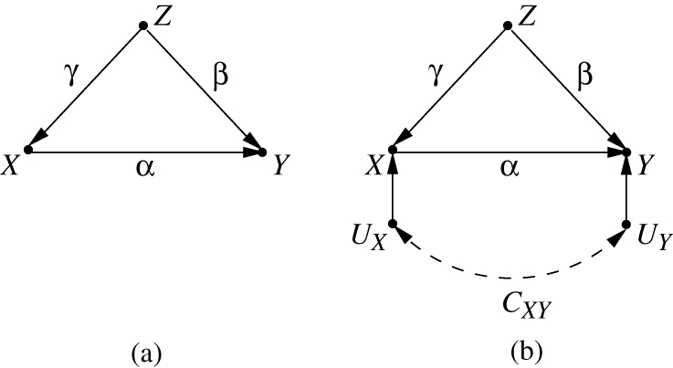
The directionality of this assignment process is captured by a path-diagram, in which the nodes represent variables, and the arrows represent the (potentially) non-zero coefficients in the equations. The diagram in Figure 1(a) represents the SEM equations of (7)–(9) and the assumption of zero correlations between the U variables,

The diagram in Figure 1(b) on the other hand represents eqs. (7)–(9) together with the assumption

while σUX,UY=CXY remains undetermined.

The coefficients α,β, and γ are called path coefficients, or structural parameters and they carry causal information. For example, α stands for the change in Y induced by raising X one unit, while keeping all other variables constant.^[2]The assumption of linearity makes this change invariant to the levels at which we keep those other variables constant, including the error variables; a property called “effect homogeneity.” Since errors (e.g., UX,UY,YZ) capture variations among individual units (i.e., subjects, samples, or situations), effect homogeneity amounts to claiming that all units react equally to any treatment, which may exclude applications with profoundly heterogeneous subpopulations.

2.4 Wright’s path-tracing rules

In 1921, the geneticist Sewall Wright developed an ingenious method by which the covariance σxy of any two variables can be determined swiftly, by mere inspection of the diagram [3]. Wright’s method consists of equating the (standardized^[3]) covariance σxy=ρxy between any pair of variables with a sum of products of path coefficients and error covariances along all d-connected paths between X and Y. A path is d-connected if it does not traverse any collider (i.e., head-to-head arrows, as in X→Y←Z).

For example, in Figure 1(a), the standardized covariance σxy is obtained by summing α with the product βγ, thus yielding σxy=α+βγ, while in Figure 1(b) we get: σxy=α+βγ+CXY. Note that for the pair X and Z, we get σxz=γ since the path X→Y←Z is not d-connected.

The method above is valid for standardized variables, namely, variables normalized to have zero mean and unit variance. For non-standardized variables the method needs to be modified slightly, multiplying the product associated with a path p by the variance of the variable that acts as the “root” for path p. For example, for Figure 1(a) we have σxy=σx2α+σz2βγ, since X serves as the root for path X→Y and Z serves as the root for X←Z→Y. In Figure 1(b), however, we get σxy=σx2α+σz2βγ+CXY where the double arrow UX↔UY serves as its own root.

2.5 Computing partial correlations using path diagrams

The reduction from partial to pair-wise correlations summarized in eqs. (4)–(6), when combined with Wright’s path-tracing rules permits us to extend the latter so as to compute partial correlations using both algebraic and path tracing methods. For example, to compute the partial regression coefficient βyx⋅z, we start with a standardized model where all variances are unity (hence σxy=ρxy=βxy), and apply eq. (6) with σx=σz=1 to get:

At this point, each pair-wise covariance can be computed from the diagram through path-tracing and, substituted in eq. (10), yields an expression for the partial regression coefficient βyx⋅z.

To witness, the pair-wise covariances for Figure 1(a) are:

Substituting in eq. (10), we get

Indeed, we know that, for a confounding-free model like Figure 1(a) the direct effect α is identifiable and given by the partial regression coefficient βxy⋅z. Repeating the same calculation on the model of Figure 1(b) yields:

leaving α non-identifiable.

2.6 Reading vanishing partials from path diagrams

When considering a set Z=Z1,Z2,…,Zk of regressors the partial correlation ρyx⋅z1,z2,…,zk can be computed by applying eq. (3) recursively. However, when the number of regressors is large, the partial correlation becomes unmanageable. Vanishing partial correlations, however, can be readily identified from the path diagram without resorting to algebraic operations. This reading, which is essential for the analysis of interventions, is facilitated through a graphical criterion called d-separation [4]. In other words, the criterion permits us to glance at the diagram and determine when a set of variables Z=Z1,Z2,…,Zk renders the equality ρyx⋅z=0.

The idea of d-separation is to associate zero correlation with separation; namely, the equality ρyx⋅z=0 would be valid whenever the set Z “separates” X and Y in the diagram. The only twist is to define separation in a way that takes proper account of the directionality of the arrows in the diagram.

Armed with the ability to read vanishing partials, we are now prepared to demonstrate some peculiarities of interventions and counterfactuals.

3.1 Interventions and their effects

Consider an experiment in which we intervene on variable X and set it to constant X=x. Let E[Y|do(x)] denote the expected value of outcome Y under such an intervention. The relationship between E[Y|do(x)] and the parameters of any given model can readily be obtained by explicating how an intervention modifies the data-generating process. In particular the intervention do(x) overrides all preexisting causes of X and, hence, transforms the graph G into a modified graph GX‾ in which all arrows entering X are eliminated, as shown in Figure 2(b).

Figure 2

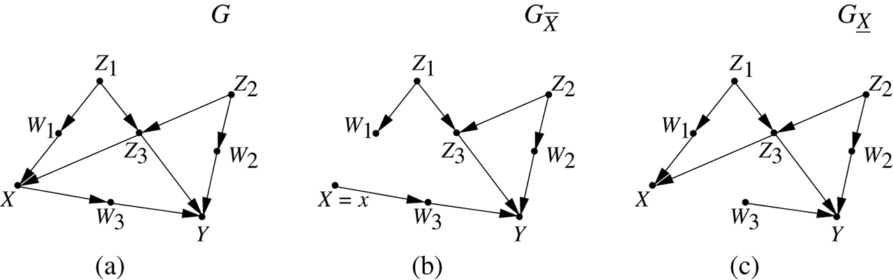
Illustrating the graphical reading of interventions. (a) The original graph. (b) The modified graph GX‾ representing the intervention do(x). (c) The modified graph GX_ in which separating X from Y represents non-confoundedness.

Thus, the interventional expectation E[Y|do(x)] is given by the conditional expectation E(Y|X=x) evaluated in the modified model GX‾. Applying Wright’s Rule to this model, we obtain a well known result in path analysis: E[Y|do(x)] = τx, where τ stands for the sum of products of path coefficients along all paths directed from X to Y.

Likewise, the average causal effect (ACE) of X on Y, defined by the difference

is a constant, independent of x, and is given by τ,

In the early days of path analysis, total effects were estimated by first estimating all path coefficients along the causal paths and then summing up products along those paths. The d-separation criterion of Definition 1 simplifies this computation significantly and leads to the following theorem.

This identification condition is known as backdoor, and it is written as (X∐Y|Z)GX_. In Figure 2(c), for example, the set Z={Z3,W2} satisfies the backdoor condition, while the set Z={Z3} does not. Note that eq. (16) is valid even if some of the parameters along the causal paths cannot be estimated. In Figure 2(c), the path coefficient along the arrow W3→Y need not be estimable, the total effect will still be given by eq. (16).

A modification of Theorem 1 is required whenever the target quantity is the direct, rather than the total effect of X on Y. In this case, the parameter α on the arrow connecting X and Y can be identified using the following Theorem ([5], Ch. 5.3.1).

In Figure 1(a), for example, the parameter α is identified by βyx⋅z because Zd-separates X from Y in Gα. In Figure 1(b), on the other hand, Z fails to d-separate X from Y in Gα and, hence, α is not identifiable by regression.

Usually, to identify a direct effect α the set Z needs to include descendants of X. For example, if α stands for the direct effect of Z3 on Y in Figure 2(a), then the set Z needs to include descendants of Z3, to block the path Z3→X→W3→Y. However, Z={X,Z2} is admissible, as well as Z={W3,W2}, but not Z={X,W3}.

A full account of identification conditions in linear systems is given in Chen and Pearl [6].

There is one more interventional concept that deserves our attention before we switch to discuss counterfactuals: covariate-specific effect. Assume we are interested in predicting the interventional expectation of Y for a subset of individuals for whom Z=z, where Z is a pre-intervention set of characteristics. We write this expectation as E[Y|do(x),z], and define it as the conditional expectation of Y, given z, in the modified post-intervention model, depicted by GX‾. Formally,

Since Z=z is pre-intervention event, it will not be affected by the intervention, so P(z|do(x))=P(z). Therefore, E[Y|do(x),z] reduces to τx+cz where c is the regression slope of Y on Z in GX‾. For example, in the model of Figure 1 we have

hence

We see that, in general, the z-specific causal effect E[Y|do(x),z] is identifiable if and only if the total effect τ is identifiable. This stands in sharp contrast to non-linear models where conditioning on Z may prevent the identification of the z-specific causal effect [7].

If however Z is affected by the intervention and our interest lies in the expected outcome of individuals currently at level Z=z had they been exposed to intervention X=x, eq. (17) no longer represents the desired quantity, and we must use counterfactual analysis instead (see Section 4.4).

3.2 The graphical representation of counterfactuals

The do-operator facilitates the estimation of average causal effects, with the average ranging either over the entire population or over the z-specific sub-population. In contrast, counterfactual analysis deals with behavior of individuals for which we have certain observations, or evidence (e). A counterfactual query asks, “Given that we observe E=e for an individual u, what would we expect the value of Y to be for that individual if X had been x?” For example, given that Joe’s salary is Y=y, what would his salary be had he had x years of education (X=x)? This expectation is denoted E[Yx|Y=y]. The conditioning event Y=y represents the observed evidence (e) while the subscript x represents a hypothetical condition specified by the counterfactual antecedent. Structural equation models are able to answer counterfactual queries of this sort, using a model modification operation similar to the do-operator.

Let  Mx stand for the modified version of M, with the equation of X replaced by X=x. The formal definition of the counterfactual Yx(u) reads

In words: The counterfactual Yx(u) in model M is defined as the solution for Y in the “surgically modified” submodel Mx. Equation (18) was called “The Fundamental Law of Counterfactuals” [8] for it allows us to take our scientific conception of reality, M, and use it to answer all counterfactual questions of the type “What would Y be had X been x?”

Equation (18) also tells us how we can find the potential outcome variable Yx in the graph. If we modify model M to obtain the submodel Mx, then the outcome variable Y in the modified model is the counterfactual Yx in the original model.

Figure 3

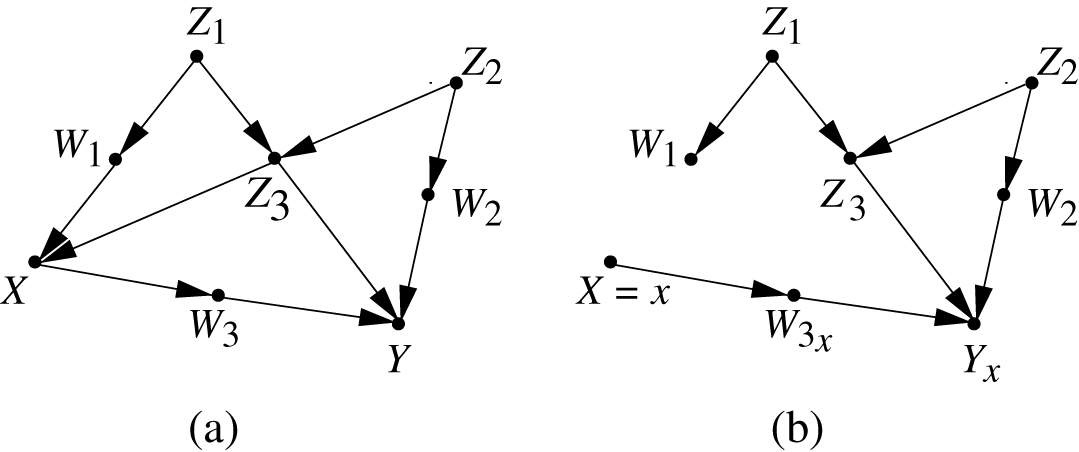
Illustrating the graphical reading of counterfactuals. (a) The original model. (b) The modified model Mx in which the node labeled Yx represents the potential outcome predicated on X=x.

Since modification calls for removing all arrows entering the variable X, as illustrated in Figure 3(b), we see that the node associated with Y serves as a surrogate for Yx, with the understanding that the substitution is valid only under the modification.

This temporary visualization of counterfactuals is sufficient to describe the statistical properties of Yx and how those properties depend on other variables in the model. In particular, the statistical variations of Yx are governed by all exogenous variables capable of influencing Y when X is held constant, as in Figure 2(b). Under such conditions, the set of variables capable of transmitting variations to Y are the parents of Y, (observed and unobserved) as well as parents of nodes on the pathways between X and Y. In Figure 2(b), for example, these parents are {Z3,W2,U3,UY}, where UY and U3, the error terms of Y and W3, are not shown in the diagram. Any set of variables that blocks a path to these parents also blocks that path to Yx, and will result therefore in a conditional independence for Yx. In particular, if we have a set Z of covariate that satisfies the backdoor criterion in M (see Definition 1), that set also blocks all paths between X and those parents, and consequently, it renders X and Yx independent in every stratum Z=z.

These considerations are summarized formally in Theorem 3.

The condition of Theorem 3, sometimes called “conditional ignorability” implies that P(Yx=y)=P(Y=y|do(X=x)) is identifiable by adjustment over Z. In other words, in linear systems, the average causal effect is given by the partial regression coefficient βyx⋅z (as in eq. (16)), whenever Z is backdoor admissible.

3.3 Counterfactuals in linear models

In linear Gaussian models any counterfactual quantity is identifiable whenever the model parameters are identified. This is because the parameters fully define the model’s functions, with the help of which we can define M and Mx in eq. (17). The question remains whether counterfactuals can be identified in observational studies, when some of the model parameters are not identified. It turns out that any counterfactual of the form E[YX=x|E=e], with e an arbitrary set of events is identified whenever E[Y|do(X=x)] is identified [5, p. 389]. The relation between the two is summarized in Theorem 4, which provides a shortcut for computing counterfactuals.

This provides an intuitive interpretation of counterfactuals in linear models: E[YX=x|E=e] can be computed by first calculating the best estimate of Y conditioned on the evidence e, E[Y|e], and then adding to it whatever change is expected in Y when X is shifted from its current best estimate, E[X|E=e], to its hypothetical value, x.

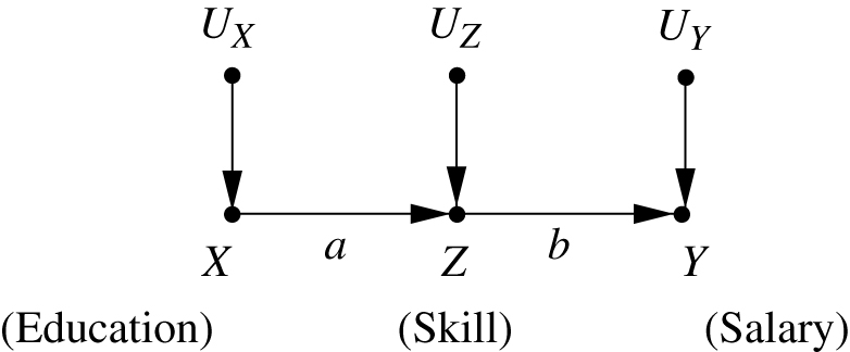
Methodologically, the importance of Theorem 4 lies in enabling researchers to answer hypothetical questions about individuals (or sets of individuals) from population data. The ramifications of this feature in legal and social contexts will be explored in the following sections. In the situation illustrated by Figure 4,

we will demonstrate how Theorem 4 can be used in computing the effect of treatment on the treated [9]

Substituting the evidence e={X=1} in eq. (20) we get:

In other words, the effect of treatment on the treated is equal to the effect of treatment on the entire population. This is a general result in linear systems that can be seen directly from eq. (20); E[Yx+1−Yx|e]=τ, independent on the evidence e. Things are different when a multiplicative (i.e., non-linear) interaction term is added to the output equation [8], but this takes us beyond the linear sphere.

4.1 The mediation fallacy

In Figure 4, the effect of X on Y consists of two parts, the direct effect, c, and the indirect effect mediated by Z, and quantified by the product ab. Attempts to disentangle the two by regression

Figure 4

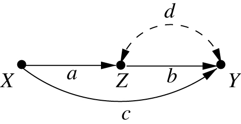
Demonstrating the mediation fallacy; “controlling for” the mediator Z does not give the direct effect c.

methods has led to a persistent fallacy among pre-causal analysts. Define the direct effect of X on Y as “the increase we would see in Y given a unit increase in X while holding Z constant,” analysts interpreted the latter as the partial regression coefficient of Y on X, controlling for Z, or

But this can’t be true because, using Wright’s rule, we get (using eq. (6)):

which coincides with c only when d=0.

The discrepancy also reveals itself through the fact that Z does not satisfy the single-door condition of Theorem (2). Conditioning on Z opens the path X→Z↔Y.

The fallacy comes about from the habit of translating “holding Z constant” to “conditioning on Z”. The correct translation is “set Z to a constant by intervention,” namely using the do-operator do(Z=z). Unfortunately statistics proper does not provide us with an operator of “holding a variable constant.” Lacking such operator, statisticians have resorted to the only operator in their disposal, conditioning, and ended up with a fallacy that has lingered on for almost a century [10, 11, 12, 13].

Thus, the correct definition of the direct effect of X on Y is (Pearl, 1998, Definition 8)

Figure 5

A model in which c cannot be estimated by one-shot OLS; it requires sequential backdoor adjustments.

Readers versed in causal mediation will recognize this expression as the “controlled direct effect” [15, 16] which, for linear systems, coincides with the natural direct effect.

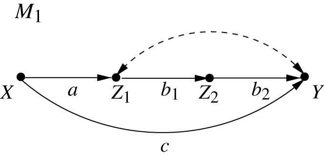
4.2 Sequential identification

It often happens that both the backdoor or single door conditions cannot be applied in one shot, but sequential application of them leads us to the right result.

Consider the problem depicted in Figure 5, in which we require to estimate the direct effect, c, in a model containing two mediators, Z1 and Z2.

Clearly, we cannot identify c by OLS, because there is no set of variables that satisfies the single door criterion relative to Gc. Conditioning on any set of mediators would open the path X→Z1↔Y. However, since the total effect is identifiable, we can write

We further notice that each of a,b1,b2 can be identified by the single door condition, using the conditioning sets:

Thus we can write

and c becomes

This problem is the linear version of the sequential decision problem treated in [17] and given a nonparametric solution using a sequential application of the backdoor condition. (See also Causality, [5, p. 352].) An attempt to solve this problem without the do-operator was made in Wermuth and Cox [18, 19] where it was called “indirect confounding” [20].

4.3 Robustness to model misspecification

In his seminal book “Introduction to Structural Equation Models” [21], Otis Duncan devotes a Chapter (8) to Specification Error. He asks: Suppose the model I used is wrong and the correct model is given by another path diagram. Can we “salvage” some of the effects estimated on the basis of the wrong model, so as to give us unbiased estimates for the true model?

Duncan was fascinated by the possibility of salvaging some unbiased estimates despite the wrongness of the working model. He goes through six different pairs of models and asks: “Show that the OLS estimator of bij [the causal parameter] in Model 1 estimates bij in Model 2 without bias.”

Duncan’s analysis was based on Wright’s rules which is not very efficient. It requires that we derive the estimates in the two models, and then compare them to decide if they are algebraically identical, in light of other model assumptions.

Using the single door criterion (Theorem 2), we can solve Duncan’s puzzle by inspection. We simply enumerate the sets of admissible covariates in each of the two models and check if there is a match.

To illustrate, consider the four models in Figure 6.

Figure 6

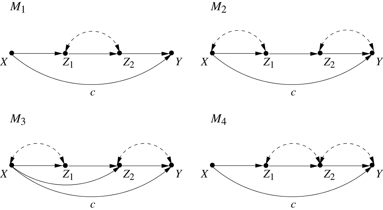
The estimate c=βyx⋅z1z2, obtained for M1, is also valid for M2 and M3, but not for M4.

Figure 7

A model demonstrating how skill-specific salary depends on education.

The admissible sets for c in each of the four models are:

1. {Z2},{Z1,Z2}

2. {Z1},{Z1,Z2}

3. {Z1,Z2}

4. none

Thus, if M1 is our working model, we can salvage our estimate of c=βyx⋅z1z2 if the true model is either M2 or M3. But if the true model is M4, there is no match to M1, and both of our options, c=βyx⋅z1z2 or c=βyx⋅z2 will be biased. M4 still permits the identification of c (using generalized instrumental variables [22]) but not by using OLS.

4.4 Mediator-specific effects

Consider the linear model depicted in Figure 7, in which X stands for education, Z for skill level and Y for salary. Suppose our aim is to estimate E[Yx|Z=z] which stands for the expected salary of individuals with current skill level Z=z, had they received X=x years of education.

Inspecting the graph, we see that salary depends only on skill level. In other words, education has no effect on salary once we know the employee’s skill level. One might surmise, therefore, that the answer is E[Yx|Z=z]=bz, independent of x. But this is the wrong answer because E[Yx|Z=z] asks not for the salary of individuals with skill Z=z but for the salary of those who currently have skill Z=z but would have attained a different skill had they obtained x years of education. The first question is captured by the expression E(Y|do(x),z) while the second is captured by the counterfactual E[Yx|Z=z]. The first evaluates indeed to bz, while the second should depends on x, since an increase in education would cause the skill level to increase beyond the current level of Z=z and, consequently, the salary would increase as well.

We now compute E[Yx|Z=z]. Using the counterfactual formula of Theorem 4

Assuming UX and UZ are standardized, we have

We see that the skill-specific salary depends on education x.

4.5 Mediator-specific effects on the treated

Consider again the model of Figure 7 and assume that we wish to assess the effect of education on salary for those individuals who have received X=x′ years of education and now possess skill Z=z. Inspecting the diagram, one might surmise again that, the salary depends on skill only, and not on the hypothetical education.

In the language of potential outcome this would amount to saying that treatment assignment is ignorable conditional on Z or Yx⊥⊥X|Z. But is it? To answer this question we set out to compute E[Yx|X=x′,Z=z] and examine whether it depends on x′ and z.

Inserting e={Z=z,X=x′} in eq. (19) we obtain

We see that E[Yx|Z=z,X=x′] depends on x′, hence ∐.

This dependence can also be seen from the graph. Recalling that Yx is none other but the exogenous variables (UZ and UY) that affect Y when X is held constant, we note that, conditioned on Z, UZ is indeed dependent on X. Hence Yx depends on X conditioned on Z; Yx∐X|Z.

4.6 Testing S-Ignorability

In generalizing experimental findings from one population (or environment) to another, a common method of estimation invokes re-calibration or re-weighting [23, 24, 25]. The reasoning goes as follows: Suppose the disparity between the two populations can be attributed to a factor S such that the potential outcomes in the two population are characterized by E(Yx|S=1) and E(Yx|S=2), respectively. If we find a set of covariates Z such that

then we can transfer the finding from population 1 to population 2 by writing

Thus, if we can measure the z-specific causal effect in population 1, the average causal effect in population 2 can be obtained by conditioning over the strata of Z and taking the average, re-weighted by P(z|S=2), the distribution of Z in the target population, where S=2.

The Achilles heal in this method is, of course, the task of finding a set Z that satisfies condition (23), sometimes called “S-ignorability.” By and large, practitioners of re-calibration methods assume S-ignorability by default and rarely justify its plausibility. Remarkably, even students of graphical models may find this condition challenging.

Consider the model in Figure 8(a).

Figure 8

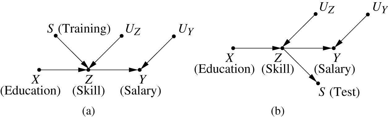
(a) The skill-specific potential outcome Yx depends on S. (b) The skill-specific potential outcome Yx is independent of S.

The structure of the model, again, shows the salary depending on skills alone, so one might surmize that eq. (23) holds. However, leveraging our graphical representation of Yx, we can easily verify that this is not the case. Since Yx is a function of {S,UZ,UY}, Z is a collider between S and UZ. Therefore, when conditioning on Z, S becomes dependent on UZ hence also on Yx. This dependence ceases to exist in Figure\ 8(b) because Z is no longer a collider. Another way to check ignorability conditions is to use Twin Networks, as in [5]. S-ignorability can also be verified algebraically using eq. (19). Substituting e={Z=z,S=s} we obtain

with c3≠0. Thus affirming the dependence of Yx on S, given Z.

References

1. Pearl J. Linear models: a useful “microscope” for causal analysis. J Causal Inference 2013;1:155–70.10.21236/ADA579021Search in Google Scholar
2. Crámer H. Mathematical methods of statistics. Princeton, NJ: Princeton University Press, 1946.Search in Google Scholar
3. Wright, S. Correlation and causation. J Agric Res 1921;20:557–85.Search in Google Scholar
4. Pearl J. Probabilistic reasoning in intelligent systems. San Mateo, CA: Morgan Kaufmann, 1988.Search in Google Scholar
5. Pearl J. Causality: models, reasoning, and inference, 2nd ed. New York: Cambridge University Press, 2009.10.1017/CBO9780511803161Search in Google Scholar
6. Chen B, Pearl J. Graphical tools for linear structural equation modeling. Los Angeles, CA: Department of Computer Science, University of California. Tech. Rep. R-432; 2015. Available at: http://ftp.cs.ucla.edu/pub/stat\_ser/r432.pdf.10.21236/ADA609131Search in Google Scholar
7. Pearl J. Detecting latent heterogeneity. Sociol Methods Res 2015. doi:10.1177/0049124115600597, Online 1–20.Search in Google Scholar
8. Pearl J, Glymour M, Jewell NP. Causal inference in statistics: a primer. New York: Wiley, 2016.Search in Google Scholar
9. Shpitser I, Pearl J. Effects of treatment on the treated: identification and generalization. Proceedings of the Twenty-Fifth Conference on Uncertainty in Artificial Intelligence. Montreal: AUAI Press, 2009:514–21.Search in Google Scholar
10. Burks B. On the inadequacy of the partial and multiple correlation technique Part I. J Exp Psychol 1926;17:532–40.10.1037/h0070156Search in Google Scholar
11. Burks B. On the inadequacy of the partial and multiple correlation technique Part II. J Exp Psychol 1926;17:625–30.10.1037/h0075654Search in Google Scholar
12. Cole S, Hernán M. Fallibility in estimating direct effects. Int J Epidemiol 2002;31:163–5.10.1093/ije/31.1.163Search in Google Scholar PubMed
13. Pearl J. Graphs causal mediation formula – a guide to the assessment of pathways and mechanisms. Prev Sci 2012;13:426–36. doi:10.1007/s11121–011–0270–1.Search in Google Scholar
14. Graphs Pearl J., causality, and structural equation models. Sociol Methods Res 1998;27:226–84.10.1177/0049124198027002004Search in Google Scholar
15. Robins J, Greenland S. Identifiability and exchangeability for direct and indirect effects. Epidemiology 1992;3:143–55.10.1097/00001648-199203000-00013Search in Google Scholar PubMed
16. Pearl J. Direct and indirect effects. In: Breese J, Koller D, editors. Proceedings of the Seventeenth Conference on Uncertainty in Artificial Intelligence. San Francisco, CA: Morgan Kaufmann, 2001:411–420.10.1145/3501714.3501736Search in Google Scholar
17. Pearl J, Robins J. Probabilistic evaluation of sequential plans from causal models with hidden variables. Uncertainty in Artificial Intelligence 11. In: Besnard P, Hanks S, editors. San Francisco, CA: Morgan Kaufmann, 1995:444–53.Search in Google Scholar
18. Cox D, Wermuth N. Distortion of effects caused by indirect confounding. Biometrika 2008;95:17–33.10.1093/biomet/asm092Search in Google Scholar
19. Wermuth N, Cox D. Graphical Markov models: overview. In: Wright J, editor. International Encyclopedia of the Social and Behavioral Sciences, vol. 10. Oxnard: Elsevier, 2014:341–50.10.1016/B978-0-08-097086-8.42048-9Search in Google Scholar
20. Pearl J. Indirect confounding and causal calculus (on three papers by Cox and Wermuth). Los Angeles, CA: Department of Computer Science, University of California. Tech. Rep. R-457; 2015.Search in Google Scholar
21. Duncan O. Introduction to structural equation models. New York: Academic Press, 1975.Search in Google Scholar
22. Brito C, Pearl J. Generalized instrumental variables. In: Darwiche A, Friedman N, editors. Uncertainty in Artificial Intelligence, Proceedings of the Eighteenth Conference. San Francisco, CA: Morgan Kaufmann, 2002; 85–93.Search in Google Scholar
23. Cole S, Stuart E. Generalizing evidence from randomized clinical trials to target populations. Am J Epidemiol 2010;172:107–115.10.1093/aje/kwq084Search in Google Scholar PubMed PubMed Central
24. Hotz VJ, Imbens GW, Mortimer JH. Predicting the efficacy of future training programs using past experiences at other locations. J Econ 2005;125:241–70.10.1016/j.jeconom.2004.04.009Search in Google Scholar
25. Pearl J, Bareinboim E. External validity: From do-calculus to transportability across populations. Stat Sci 2014;29:579–95.10.21236/ADA563868Search in Google Scholar
© 2017 Walter de Gruyter GmbH, Berlin/Boston
Articles in the same Issue
- Research Articles
- Design and Analysis of Experiments in Networks: Reducing Bias from Interference
- Interventional Approach for Path-Specific Effects
- Entropy Balancing is Doubly Robust
- Semi-Parametric Estimation and Inference for the Mean Outcome of the Single Time-Point Intervention in a Causally Connected Population
- Identification of the Joint Effect of a Dynamic Treatment Intervention and a Stochastic Monitoring Intervention Under the No Direct Effect Assumption
- Causal, Casual and Curious