Adjustment models for multivariate geodetic time series with vector-autoregressive errors
-
Boris Kargoll

 ,
Alexander Dorndorf
,
Mohammad Omidalizarandi
,
Jens-André Paffenholz
and
Hamza Alkhatib
,
Alexander Dorndorf
,
Mohammad Omidalizarandi
,
Jens-André Paffenholz
and
Hamza Alkhatib

Abstract
In this contribution, a vector-autoregressive (VAR) process with multivariate t-distributed random deviations is incorporated into the Gauss-Helmert model (GHM), resulting in an innovative adjustment model. This model is versatile since it allows for a wide range of functional models, unknown forms of auto- and cross-correlations, and outlier patterns. Subsequently, a computationally convenient iteratively reweighted least squares method based on an expectation maximization algorithm is derived in order to estimate the parameters of the functional model, the unknown coefficients of the VAR process, the cofactor matrix, and the degree of freedom of the t-distribution. The proposed method is validated in terms of its estimation bias and convergence behavior by means of a Monte Carlo simulation based on a GHM of a circle in two dimensions. The methodology is applied in two different fields of application within engineering geodesy: In the first scenario, the offset and linear drift of a noisy accelerometer are estimated based on a Gauss-Markov model with VAR and multivariate t-distributed errors, as a special case of the proposed GHM. In the second scenario real laser tracker measurements with outliers are adjusted to estimate the parameters of a sphere employing the proposed GHM with VAR and multivariate t-distributed errors. For both scenarios the estimated parameters of the fitted VAR model and multivariate t-distribution are analyzed for evidence of auto- or cross-correlations and deviation from a normal distribution regarding the measurement noise.
1 Introduction
Geodetic observation models of surveyed phenomena often include unknown quantities in terms of parameters to be estimated by adjustment computations. The most general structure of observation model is described by non-linear condition equations in which multiple observations and unknown parameters may be linked to each other [1]. This general case of adjustment calculus was called Gauss-Helmert model (GHM) by Wolf [2]. There exist numerous special cases of this model that have been studied extensively, e. g., the errors-in-variables (EIV) model adjusted by the method of total least squares [3] or by its various generalizations [4], [5], [6], [7]. Another special case of the GHM is the Gauss-Markov model (GMM), in which the observations are still linked to functional model parameters but occur in separate equations [8], [9], [10]. Such models may also contain variance-covariance information about the measurements; this information defines the so-called stochastic model. Since adjustment calculus has been elaborated on the basis of matrix calculus, variance-covariance information regarding the observables is usually arranged as a matrix, called the “variance-covariance matrix” (VCM).
Since the dimension of the VCM equals the number of observations, the storage and processing of this matrix in the course of the adjustment computations can be challenging, especially because modern sensors such as accelerometers, laser scanners, laser tracker or satellite-based sensors tend to provide huge data sets consisting of millions or even billions of observations even within relatively short periods of time. It is usually not an option to omit the variance-covariance information within the adjustment computations since the standard parameter estimators lose desirable quality characteristics when this information is neglected. For instance, the least-squares-estimator in the GMM ceases to be the best linear unbiased estimator (BLUE) when the VCM is dropped in the estimation equation [11]. Furthermore, it is often desirable in geodetic data analysis to obtain a realistic description of the uncertainties or variance-covariance information of the estimated parameters, which information is unavailable when an adequate stochastic model of the observables is missing. The “curse of dimensionality” concerning the VCM is aggravated by the increasingly practiced combination of multiple observation series stemming, e. g., from 3D sensors or from sensor networks. Time series of such measurements, e. g., GPS and laser scanner measurements, frequently have been found to be correlated in such a way that the VCM is fully populated, e. g., [12], [13], [17], [16], [14], [15].
To alleviate the computational burden or even computational infeasibility in connection with the storage and processing of a huge VCM, an alternative approach to the stochastic modeling of variance-covariance information can be applied. The goal of that approach is to fully de-correlate the observables by transforming the observation model in such a way that the VCM of the transformed observables becomes a diagonal matrix, e. g., the identity matrix [18]. A diagonal VCM can easily be handled within the adjustment procedure [19], e. g., through vectorization of the occurring matrix products. In geodetic applications the correlations of the observables may frequently be described as colored noise [20], in which case the stochastic model can be expressed as an autoregressive (AR) or autoregressive moving average (ARMA) process and the transformation of the observation equations achieved by means of a computationally efficient digital de-correlation filter [21], [22]. Such processes have also been estimated by means of total least squares based on an EIV model [23]. To model auto- and cross-correlations of multivariate time series, the aforementioned AR and ARMA processes have been extended to vector-autoregressive (VAR) and vector-autoregressive moving average (VARMA) processes [24]. The model order of these recursive processes can be specified to define how far the correlations reach into the past. Thus, VAR(MA) processes can be used to model quite detailed patterns of auto- and cross-correlations. The innovation of the current contribution is to incorporate VAR processes into the GHM as colored noise models.
The white-noise components of (V)AR or (V)ARMA processes are usually assumed to be normally distributed. However, this assumption may be unrealistic or at least questionable in a practical situation, e. g., due to numerous outliers afflicting the measurements. It may then be safer to replace the normal distribution by a larger family of distributions defined by probability density functions having thicker tails than the “ideal” normal distributions. For instance, the usage of generalized t-distributions and of scaled t-distributions has been proposed in connection with ARMA processes [25]. The scaled, multivariate t-distributions have also been applied in connection with VAR processes within rather simple GMM [26], [27]. A key feature of using multivariate t-distributions is that the associated degree of freedom (df) can be estimated alongside the functional parameters, the VAR coefficients and the scale or cofactor matrix; such a method may be called a self-tuning estimator [28] since it does not involve a tuning constant for classifying the in- and outliers, in contrast to for instance Huber’s M-estimator [29]. The df provides evidence of deviations of the measurements’ actual probability distribution from a normal distribution: For large df the multivariate t-distribution is similar to a multivariate normal distribution, whereas the t-distribution has much thicker tails than the latter for a small df, which may indicate the presence of numerous outliers.
The estimation procedure is implemented as an iteratively reweighted least-squares (IRLS) method. The weights are treated as random variables, which are numerically determined by the expectation step within an expectation maximization (EM) algorithm [30]. The various types of model parameters are estimated group-by-group within the maximization step. To deal with the condition equations within the GHM, constrained EM in the spirit of [31] is applied. Due to the down-weighting of observations with extreme errors,[1] this method can be expected to yield a robust estimator for the GHM. Koch introduced the GHM with t-distributed errors and subsequently extended the model to include variance components [32], [33]. This type of GHM is now extended to include a VAR model with multivariate-t-distributed errors. This yields an approach complementary to that of modeling a small number of outliers as additive, unknown offsets within the afflicted observations, as done in [34], [35]. Therefore, the proposed adjustment model is directed at applications in which rather large numbers of outliers can be expected. To model the auto- and cross-correlations, we do not employ the more general VARMA processes since we found the estimation of the moving average part by means of an EM algorithm to diverge.
The paper is structured as follows. In Section 2, we specify the multivariate observation model, the correlation model, and the stochastic model, which jointly define the GHM with VAR and multivariate t-distributed errors. In Section 3, we formulate the optimization principle employed to adjust this model, and we derive the normal equations to be solved within the EM algorithm. We show that this algorithm estimates the functional parameters, the VAR coefficients and the parameters defining the multivariate t-distribution essentially via IRLS. The Monte Carlo simulation described in Section 4 serves the purpose of validating the algorithm, by showing the biases to be expected in the practical situation of data approximation by a circle based on a GHM with VAR and multivariate t-distributed errors. In Section 5 we demonstrate the application of the algorithm for the adjustment of a real, multivariate accelerometer data set, whose offset and drift are modeled as part of a GMM (viewed as a special case of the GHM) with VAR and multivariate t-distributed errors. In a second applied scenario real laser tracker measurements with outliers are adjusted to estimate the parameters of a sphere employing the proposed GHM with VAR and multivariate t-distributed errors. Finally, some limitations and consequently potential extensions of the presented methodology to be explored in the future are outlined in the conclusions and outlook.
2 Adjustment models for multivariate time series
The purpose of this section is to develop adjustment models suitable for the fitting of multivariate geodetic time series. According to the standard categorization in geodetic adjustment theory these models have two main components: the deterministic model and the stochastic model. The following sub-sections demonstrate some possible structures of these models that have been found useful in geodetic time series analysis. These structures allow for certain generalizations of the standard GHM and GHM by allowing their random deviations to be auto- and cross-correlated through (V)AR processes while potential deviations from a normal distribution are modeled stochastically by a multivariate t-distribution.
2.1 Structures of the deterministic observation model
2.1.1 Deterministic part of the Gauss-Helmert model
We suppose that N time series are observed simultaneously without gaps, so that each series consists of n measurements. The measurements can then be doubly indexed in the form
Each type of quantity in these equations can be vectorized in different ways to obtain more compact notations. The rule will be that all column vectors are symbolized by bold-faced, lower-case Greek letters (in case of unknown parameters) or Roman letters. Firstly, the quantities of one type occurring throughout the time series
to define the multivariate observation time series
Secondly, the observations, location parameters and random deviations can be grouped series-by-series for
to define the observation series
Note that the additional colons are used to distinguish the two types of vectors, e. g., the observations
so that (3) turns into the single vector equation
Note that the relationship
Note also that the vectors
where the
of the
beginning with
In practice the goal usually is to fit a specific functional model to the given measurements, e. g., a circle. Such a model generally depends on unknown parameters
This equation and (7) form the deterministic part of the GHM, which was defined similarly in [32]. The given somewhat unusual notation, especially the introduction of location parameters, in the setup of the GHM is more aligned with the method of constrained ML estimation than with the usual method of LS. The former estimation method will be more suitable than the latter in connection with the estimation of VAR models and usage of a non-Gaussian pdf.
2.1.2 Deterministic part of the Gauss-Markov model
With certain kinds of adjustment problems each location parameter
Then, the observation equations (1) take the form
Vectorizing the (unknown) function values
or by time series as
or collectively, by vectorizing
This structure of observation equation defines the GMM. Using (14), the condition equations (13) are then simply taken as
where the “corrections” v are related to the random deviations e via sign reversal. In view of the additional stochastic model imposed on the observation model later on, the representation (18) is preferred in this paper. In case the function f can be written as a matrix-vector product
instead of (18). Linear models have been studied thoroughly in mathematical statistics and geodesy [36], [18]. The parameters
2.2 Stochastic modeling
2.2.1 Modeling of correlations using vector-autoregressive processes
The simplest case of a stochastic model occurs for uncorrelated observables with identical variances, so that the VCM Σ is the rescaled identity matrix
for some
where
2.2.2 Modeling of observational weights using multivariate t-distributions
Another standard decomposition of a the VCM Σ is given in terms of the “weight matrix” P by
The main diagonal of the VCM Σ consists of the variances of the individual observables, whereas the main diagonal elements of P are commonly referred to as “weights”. The meaning of the weights is twofold in practice: On the one hand, weights may be interpreted as “repetition numbers”, i. e., as the number of times that the corresponding observations have occurred. On the other hand, weights can be assigned to observations in order to diminish or increase their relative importance and influence in statistical inference. Abnormal or extreme observations (“outliers”), located in the tails of the probability density function (pdf) defining their probability distribution, are frequently encountered in geodetic data analysis. One standard approach to handling such observations consists in their “down-weighting” by giving them lesser weights than non-outliers (“inliers”). Alternatively, it is possible to carry out statistical tests in order to identify and delete outlying observations (e. g., [39], [40], [41]). However, the deletion of observations creates data gaps, which prohibit the usage of recursive time series models, such as the VAR processes considered in Sect. 2.2.1. Therefore, we restrict ourselves to the approach based on the down-weighting of outlying observations, which avoids their elimination and consequential data gaps. Since the data sets analyzed nowadays tend to be huge and oftentimes have stochastic properties unknown to the practitioner, it is necessary to have a data-adaptive and computationally efficient procedure for computing weights at hand. Mathematically, such a procedure is based on a function (the “weight function”), which corresponds to a certain pdf of the random deviations.
For the purpose of multivariate modeling including potential cross-correlations, the well-known Student’s t-distribution can be generalized to an N-variate t-distribution
Since the scale matrix Ψ is related to the VCM via
(see also [44]). The joint pdf of n such white noise vectors
This pdf is more intricate and therefore more difficult to handle in maximum likelihood (ML) estimation than the pdf of a multivariate normal distribution. However, it is well known that a multivariate t-distributed random vector
and
It can be seen in (28) that the white noise vector
Under the distributional assumptions (28)–(29) the joint pdf of white noise vectors
and (27) defines the corresponding marginal distribution of
2.3 Representations of the adjustment models as likelihood functions
A likelihood function L can be defined by a pdf by fixing an element of its domain (the observation space) and by letting its parameters be “variables”. The pdf (30) directly involves as parameters the entries of the cofactor matrix Ψ and the df ν. When certain realizations
where
Consequently, (31) can be recast as
Here, for brevity of expressions, we defined the so-called lag polynomial
Thus, the pdf (30) indirectly depends also on the VAR coefficients in the matrices
To fix the dimensions of the parameter space, the kth rows of the VAR coefficient matrices are combined to column vectors of length
which in turn are combined to the single column vector
of length
and
Taking the natural logarithm of the pdf (30) with
A similar log-likelihood involving multiple (univariate) AR processes instead of a single (multivariate) VAR process was established in [46]. To obtain the log-likelihood function
3 Estimation
Maximum likelihood estimation of the model parameters
The Q-function for the GHM with VAR and multivariate t-distributed errors is given by (82) in the Appendix. Evaluation of the conditional expectation of the random weight variables
The tilde on the conditional expectation
which involves as additional parameters an
for some numerically fixed matrix X, matrix B and vector m, linearization
is applied as shown for instance in [32]. Here, we define the
the
the
the
and the
Whereas
the normal equations for the incremental functional parameters
(48)the normal equations for the location parameters
(49)denoting
(50)(51)the normal equations for the VAR coefficient matrices
(52)denoting
(53)with
the normal equations for the inverse cofactor matrix
(54)the normal equation for the df ν (cf. Sect. 5.8.2 [47]):
(55)involving the digamma function
the normal equations for the Lagrange multipliers
(56)
(supposing that the inverse exists), these parameters can be eliminated from (56) via substitution, which results in
Together with (48), this gives the normal equation system
The parameter groups
Having completed s iterations, the first ECM-step of the new iteration
from (59), where the unknown matrices Ψ and
are fixed by substituting (i. e., “conditioning on”) the previous solutions
Moreover, the new solution
via substitution into the rearranged equation (43).
The solution
Next, the new solution
of the VAR coefficient matrices is computed from (52), based on the new correlated residuals
computed from the model (7) and the corresponding residual matrix
with the usual boundary values
in view of (33) and (64). Conditional on these values, equation system (54) gives rise to the solution for the cofactor matrix
Finally,
where
Equation (68) is obtained by defining the log-likelihood function directly on the joint pdf (30) of the white-noise series based on the multivariate t-distribution, and setting its partial derivative with respect to ν equal to zero. This modification of the ECM algorithm has been called ECM either (ECME) [49], [50]. The zero search can be performed with mathematical standard software such as the INTLAB library ([51]) or using a grid search. The estimation of the df concludes the current M-step. The E- and M-step (in the form of an ECME algorithm) are repeated until certain stop criteria are fulfilled, e. g., a combination of a maximum number of iterations and thresholds
for the minimum absolute difference between the current and the previous solution. We defined the threshold
4 Results
4.1 Gauss-Helmert model: Adjustment of simulated data of a 2D circle
In the first part of this section, the performance of the EM algorithm derived in previous Sect. 3 in producing correct estimates within a Monte Carlo (MC) simulation is studied. For this purpose, generated measurements of
On the one hand, the vector
On the other hand, the vector
where n was set to 250, 500, 2500 and 5000 in different simulation runs. For greater clarity of notation, we write
with
Thus, the measurements are equidistantly distributed along the circle, and one half of the circle was measured twice. The numerical realizations
where random numbers
with
In total 500 MC samples of the white-noise components for stochastic model A and B as well as for the different sample sizes n were randomly generated using MATLAB’s mvtrnd routine. The resulting simulated observations in models A and B were then adjusted by means of the EM algorithm. The maximum number of iterations was set to
4.1.1 Analysis of the simplified stochastic model on the estimation results
The results of this comparison are visualized in Fig. 1 and Fig. 2 by means of box plots. In each box plot, the middle line shows the median. The bottom and the top border of the boxes are the 25th percentile (Q1) and 75th percentile (Q3), respectively. The distance Q3-Q1 is the inter-quartile range (IQR). The additional lines above and below the box are the whiskers defined by
The statistical moments of the calculated bias
4.1.2 Analysis of the degree of freedom on the estimation results
The influence of the df on the estimation results using the EM algorithm is displayed in Fig. 3 and Fig. 4. Figure 3 shows the estimated

MC simulation results of the estimated parameters for stochastic model A. Dash line: true value of simulation.

MC simulation results of the estimated VCM for stochastic model A.

Comparison of the MC simulation results between the stochastic model A and B. The maximum deviation of

Comparison of VAR coefficients between the MC simulation results of stochastic model A and B.
Statistics of MC simulation results for the bias of the estimated parameters
| LS Model A | EM Model A | EM Model B | |
| mean | |||
| std | |||
| minimum | |||
| maximum | |||
| 95 % interval | |||
| mean | |||
| std | |||
| minimum | |||
| maximum | |||
| 95 % interval | |||
| mean | |||
| std | |||
| minimum | |||
| maximum | |||
| 95 % interval | |||
| mean | |||
| std | |||
| minimum | |||
| maximum | |||
| 95 % interval | |||
| mean | |||
| std | |||
| minimum | |||
| maximum | |||
| 95 % interval | |||
| mean | |||
| std | |||
| minimum | |||
| maximum | |||
| 95 % interval |
Statistics of MC simulation results for the bias of the estimated parameters
| EM Model A | EM Model B | |
| mean | 2.25 | 0.44 |
| std | 0.21 | 0.21 |
| minimum | 1.70 | −0.19 |
| maximum | 3.12 | 1.16 |
| 95 % interval | ||
| mean | ||
| std | ||
| minimum | ||
| maximum | ||
| 95 % interval | ||
| mean | ||
| std | ||
| minimum | ||
| maximum | ||
| 95 % interval | ||
| mean | ||
| std | ||
| minimum | ||
| maximum | ||
| 95 % interval | ||
| mean | ||
| std | ||
| minimum | ||
| maximum | ||
| 95 % interval |
4.2 Gauss-Markov model: Adjustment of 3D MEMS accelerometer data
In the second part of this section, the performance of the EM algorithm elaborated in Sect. 3 (which we also refer to as “VAR-multivariate algorithm” in the following) is studied on real data sets, which were measured by an accelerometer. Cost-effective Micro-Electro-Mechanical-Systems (MEMS) accelerometers have received increasing attention in numerous applications such as vibration analysis of bridge structures, e. g., [52], [53], [54]. In such applications, it is desirable to select a suitable accelerometer by considering, for instance, measurement and sensitivity ranges, uncertainty of measurements, cost, and sampling rate. [55] proposed a two-step scenario to accomplish the suitability analysis for MEMS accelerometers. Firstly, the calibration of the MEMS accelerometers was carried out for different positions and over different temperature ranges. Therefore, the characteristics of the calibration parameters such as biases, scale factors and non-orthogonalities between axes have been inspected during different temperature changes. Secondly, a controlled excitation experiment was conducted using a shaker to compare and validate estimated harmonic oscillation parameters including frequency, amplitude and phase shift with other MEMS accelerometers as well as a high-end reference accelerometer. The second step additionally allowed to check the time synchronization between the MEMS accelerometers. Later on [54] extended the aforementioned two-step scenario to three-step scenario. In the third-step, a static test experiment was accomplished over a long period of time, which allows to estimate an offset and a drift of the measurements as well as auto-correlations and underlying distributional parameters for each axis individually.
As part of this study and to make the third step of the aforementioned three-step scenario more comprehensive, the (unknown) auto- as well as cross-correlations and the (unknown) distributional characteristics of the acceleration measurements recorded from three different axes are analyzed by employing VAR models with t-distributed errors. For this purpose, acceleration measurements were recorded from a cost-effective MEMS accelerometer of type BNO055 with Arduino UNO-Board and 9 axes motion shield (produced from Bosch GmbH), which is a so-called NAMS. The measurements were carried out in three different axes over a period of 24 hours (Fig. 5) with a sampling frequency of 0.3789 Hz. Although it is possible to perform the measurements with a higher sampling frequency (e. g., up to 200 Hz), the aforementioned sampling frequency is specified to speed up the processing.
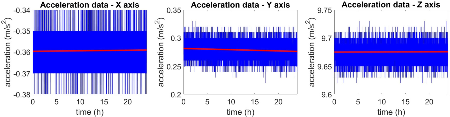
Raw acceleration data recorded from the MEMS accelerometer of type NAMS (blue) and fitted linear model (red) estimated from VAR-multivariate algorithms.
An observation model consisting of (1) a functional model based on a linear drift with an unknown offset (intercept) and a linear drift coefficient, (2) an auto- and cross-correlation model based on a VAR process with unknown model order and coefficients, and (3) a stochastic model based on the multivariate t-distribution with unknown scale matrix and df. This observation model has the structure of the GMM with VAR and t-distributed errors. The maximum number of iterations is set to
where the vector
where
which has full rank.
Statistics of the estimated unknown parameters in the functional model based on the linear drift model, the auto- and cross-correlation model based on the VAR process and the stochastic model based on the centered and scaled t-distribution with an unknown degree of freedom and unknown scale factor from the AR-univariate and VAR-multivariate algorithms.
| Sensor | Method | Axis | p | WNT | |||||
| [ |
[ |
[ |
[–] | [–] | [–] | [–] | |||
| NAMS | multivar. | x | −0.3598 | 4.80e-09 | 0.0224 | 1 | – | yes | 2.1 |
| y | 0.2810 | −6.11e-08 | 0.0493 | – | |||||
| z | 9.6752 | 4.63e-09 | 0.0534 | – | |||||
| univar. | x | −0.3597 | 6.81e-09 | 0.0066 | 1 | −6.2927e-04 | yes | 16.87 | |
| univar. | y | 0.2811 | −6.12e-08 | 0.0132 | 1 | 0.0013 | yes | 120 | |
| univar. | z | 9.6746 | 6.65e-09 | 0.0141 | 1 | 0.0087 | yes | 120 |
Table 3 summarizes the statistics of the estimated parameters from the VAR-multivariate and AR-univariate algorithms based on the GMM.
Fig. 6 (a) illustrates the estimated p-values for different VAR model orders. The estimated p-values are all above the significance level, and thus, the VAR model order 1 is selected. Fig. 7 (b) shows the calculated test values that are compared with the cumulative distribution function of the chi-square distribution (

Results of the portmanteau test (p-value) for VAR model orders
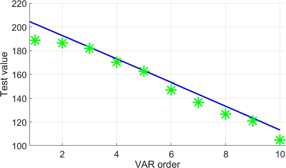
Results of the test values for VAR model orders
The estimated VCM (Σ) and its corresponding correlation matrix (
according to the definition of the VAR coefficient matrix (23). As it could be seen, the VAR model coefficients corresponding to y and z axes are slightly greater than those for the x-axis. In addition, the estimated colored and white noise residuals obtained from NAMS acceleration data are illustrated in Fig. 8. The subtraction of the aforementioned residuals are provided (Fig. 9) to have a better realization of the amplitude of the colored noise residuals at each axis. As it could be seen, the y and z-axes of the NAMS accelerometer have stronger colored measurement noise in comparison to the x-axis.

Representation of the estimated colored and white noise residuals (x, y, and z axes in a sequence) obtained from NAMS acceleration data for VAR model order 1.

Differences of the estimated residuals (x, y, and z axes in a sequence) (b).
The proposed approach in this study assists us to select a proper MEMS accelerometer for, e. g., the purpose of vibration analysis of bridge structures. It is applied as a third step of the aforementioned scenario in the suitability analysis of the MEMS accelerometer by providing information about unknown offset and drift coefficients, VAR model order and stochastic model parameters. Therefore, a sensor with possibly less offset and drift coefficients over a long period as well as lower uncertainty of the measurements could be selected. In addition, a minimum VAR model order between different MEMS accelerometers reveals less cross-correlation between their axes, which can also be considered as an important influencing factor in the selection procedure. Moreover, it is observed that the MEMS accelerometers used in this study have minimum standard deviations in the x-axis compared to the two other axes. Therefore, the sensors should be mounted with their x-axis in the main observations direction during the monitoring of bridge structures.
4.3 Gauss-Helmert model: Adjustment of a sphere from continuous laser tracker measurements
In the third part of this section, the performance of the EM algorithm in a real-world application estimating the parameters
which is an extension in 3D space by considering the z-component in addition to the nonlinear equation of the 2D circle in (70).
To illustrate and discuss the adjustment of a sphere, 3D coordinates on the surface of a sphere with known radius were obtained by continuous measurements with 10 Hz using a laser tracker of type Leica AT960-LR. The extended uncertainty of the x-, y- and z-coordinate is given by
4.3.1 Analysis of the measurements
In analogy to the analysis scheme for the simulated 2D circle in Sect. 4.1, the sphere parameters are obtained on the one hand by means of a LS estimation, i. e. a classical GHM, and on the other hand by means of the proposed EM algorithm in this contribution. The thresholds used within the EM algorithm are similar to the simulation. In this real-world application study, the multivariate portmanteau test is applied to select an adequate VAR model order p by testing the estimated residuals

Results of the test values for VAR model orders
Before discussing the results of the parameter estimation, we will discuss the results of the portmanteau test in Fig. 10. The blue line indicate the critical value for the significance level
4.3.2 Discussion of the results
The estimated parameters
Estimated sphere parameters for the LS model and the VAR model orders
| LS Model | EM Model |
EM Model |
|
| 99.317 | 99.317 | 99.317 | |
| 4014.130 | 4014.129 | 4014.125 | |
| 4.009 | 4.009 | 4.006 | |
| 68.943 | 68.943 | 68.939 | |
| – | |||
| − | 2.60 | 2.10 | |

Estimated colored and white noise residuals obtained from laser tracker measurements for VAR model order
Figure 11 depicts the estimated colored and white noise residuals obtained from laser tracker measurements for VAR model order
The red circles in Fig. 11 indicate white noise and the green dots indicate the weighted white noise, i. e. white noise values multiplied with their weights
Table 5 shows the results of the VAR coefficients for the model orders
Taking a look at the VAR coefficients for the model order
Results of the VAR coefficients for the VAR models of order
| EM Model |
EM Model |
EM Model |
|
| – | |||
| – | – |
5 Conclusions and outlook
The nonlinear Gauss-Helmert model constitutes the most general adjustment model, which is widely used in geodesy. This model consists of condition equations (which link the observations and the functional parameters occurring in the mathematical model employed to approximate the measurements) and of a stochastic model. The latter usually is defined by a VCM, which tends to be huge when the number of measurements is large. We therefore applied and investigated, in the context of multivariate time series, a more manageable type of stochastic model defined by a vector autoregressive (VAR) process. This model takes both auto- and cross-correlations into account and can be estimated alongside the functional model parameters. By employing a multivariate t-distribution with data-adaptable scale matrix and degree of freedom, moderate deviations from the usual assumption of normally distributed noise are possible. To fuse this t-distribution with the VAR process and the constraints, we applied the idea of formulating a generalized Gauss-Helmert model in terms of a likelihood function, which is maximized under the constraints. The proposed model allows for a computationally convenient iteratively reweighted least-squares method based on a constrained expectation maximization algorithm. This methodology extends the previously established approach involving univariate autoregressive models that ignored potential cross-correlations between the time series. Analysis of the biases by means of Monte Carlo simulations showed that the functional model parameters tend to be highly accurate when the number of observations is increased, whereas a significant bias of the degree of freedom of the multivariate t-distribution persists, in particular for smaller degrees of freedom. The accuracy of the estimated VAR coefficients and of the scale parameters generally improves with larger datasets. The methodology is also applicable to functional models that take the form of a Gauss-Markov model, as shown by an analysis of real accelerometer data modeled by an offset and a linear drift. For another real-world application, which utilizes continuous measurements of a laser tracker on a sphere, the applicability of the proposed Gauss-Helmert model was also demonstrated. Furthermore, the analyses of the results for this application demonstrated that the estimated VAR process coefficients and the estimated parameters of the multivariate t-distribution allows for detailed evaluations of the auto- and cross-correlation as well as the distributional characteristics of the measurement noise. Thus, actual deviations of the noise from expected white-noise and normal-distribution behavior become visible in the course of adjusting real-world datasets. Due to its flexibility the proposed innovative type of Gauss-Helmert model with VAR and t-distributed errors could be useful in various fields of geodesy such as engineering geodesy or Earth system modeling where multivariate, functionally complex and correlated time series are analyzed. Since such datasets often contain gaps a further extension of the model and EM algorithms such that the E-step yields also values for missing measurement values appears to be useful. It is also conceivable that the VAR processes of the current model are replaced by other stochastic processes that might match the correlation pattern of a given set of observables better.
Funding source: Deutsche Forschungsgemeinschaft
Award Identifier / Grant number: 386369985
Funding statement: This research was supported by the Deutsche Forschungsgemeinschaft (DFG, German Research Foundation) – project number 386369985.
Appendix A Derivations
Log-likelihood and Q-functions
Here, the conditional expectations
and
with
The following normal equations can be derived from the linearized Lagrangian (obtained by combining (40) with (42))
by applying slight modifications to the steps concerning the GMM with VAR and multivariate t-distributed errors given in Appendix B in [26], using (8).
Normal equations for the location parameters
Applying (8) to eliminate the time dependence of the location parameters
Normal equations for the VAR coefficient matrices
Substituting (32) into (86) for brevity of expressions and applying also Eq. (88) in [59],
The joint normal equation system for all of the VAR coefficient matrices
Normal equations for the inverse scale matrix
Substituting (33) into (86) for brevity of expressions and applying the arguments given in Sect. 373 in [18], one obtains
Acknowledgments
The authors would like to acknowledge ALLSAT GmbH for providing the low-cost MEMS sensor used in the experiments. In addition, the authors would also like to acknowledge Eva Kemkes, M. Sc. (ALLSAT GmbH) for her assistance in data acquisition within the experiments.
-
Author contributions: Conceptualization, B. K., H. A., J.-A. P., A. D., M. O.; methodology, B. K., H. A. and A. D.; software, B. K., A. D., M. O. and H. A.; validation, H. A., A. D. and M. O.; formal analysis, A. D., M. O. and H. A.; investigation, B. K., A. D., M. O., J.-A. P., H. A.; resources, B. K.; data curation, A. D.; writing–original draft preparation, B. K., A. D., M. O., H. A. and J.-A. P.; writing–review and editing, B. K., H. A. and J.-A. P.; visualization, H. A., A. D. and M. O.; supervision, B. K., H. A. and J.-A. P.; project administration, B. K., H. A. and J.-A. P.; funding acquisition, B. K., H. A. and J.-A. P.
References
[1] Helmert FR. Die Ausgleichungsrechnung nach der Methode der kleinsten Quadrate. Leipzig, Teubner, 1872.Search in Google Scholar
[2] Wolf H. Das geodätische Gauß-Helmert-Modell und seine Eigenschaften. Z Vermessungswesen 1978, 103, 41–43.Search in Google Scholar
[3] Golub GH, Van Loan CH. An analysis of the total least squares problem. SIAM J Numer Anal 1980, 17, 883–893.10.1137/0717073Search in Google Scholar
[4] Schaffrin B, Wieser A. On weighted total least-squares adjustment for linear regression. J Geod 2008, 82, 415–421.10.1007/s00190-007-0190-9Search in Google Scholar
[5] Neitzel F. Generalization of total least-squares on example of unweighted and weighted 2D similarity transformation. J Geod 2010, 84, 751–762.10.1007/s00190-010-0408-0Search in Google Scholar
[6] Xu P, Liu J, Shi C. Total least squares adjustment in partial errors-in-variables models: algorithm and statistical analysis. J Geod 2012, 86, 661–675.10.1007/s00190-012-0552-9Search in Google Scholar
[7] Amiri-Simkooei A, Jazaeri S. Weighted total least squares formulated by standard least squares theory. J Geodetic Sci 2012, 2, 113–124.10.2478/v10156-011-0036-5Search in Google Scholar
[8] Gauß CF. Theoria Motus Corporum Coelestium. Hamburg, Perthes und Besser, 1809.Search in Google Scholar
[9] Gauß CF. Theoria Combinationis Observationum. Göttingen, Dieterich, 1823.Search in Google Scholar
[10] Markov AA. Wahrscheinlichkeitsrechnung. Leipzig, Teubner, 1912.Search in Google Scholar
[11] Aitken AC. On least squares and linear combinations of observations. Proc Royal Soc Edinburgh 1935, 55, 42–48.10.1017/S0370164600014346Search in Google Scholar
[12] Amiri-Simkooei AR. Noise in multivariate GPS position time-series. J Geod 2009, 83, 175–187.10.1007/s00190-008-0251-8Search in Google Scholar
[13] Koch KR, Kuhlmann H, Schuh WD. Approximating covariance matrices estimated in multivariate models by estimated auto- and cross-covariances. J Geod 2010, 84, 383–397.10.1007/s00190-010-0375-5Search in Google Scholar
[14] Kermarrec G, Schön S. Fully populated VCM or the hidden parameter. J Geod Sci 2017, 7, 151–161.10.1515/jogs-2017-0016Search in Google Scholar
[15] Kermarrec G, Schön S. A priori fully populated covariance matrices in least-squares adjustment—case study: GPS relative positioning. J Geod 2017, 91, 465–484.10.1007/s00190-016-0976-8Search in Google Scholar
[16] Kauker S, Schwieger V. A synthetic covariance matrix for monitoring by terrestrial laser scanning. J Appl Geod 2017, 11, 77–87.10.1515/jag-2016-0026Search in Google Scholar
[17] Kauker S, Holst C, Schwieger V, Kuhlmann H, Schön S. Spatio-temporal correlations of terrestrial laser scanning. AVN 2016, 123, 170–182.Search in Google Scholar
[18] Koch KR. Parameter Estimation and hypothesis testing in linear models. Berlin, Springer, 1999.10.1007/978-3-662-03976-2Search in Google Scholar
[19] Kermarrec G, Schön S. Taking correlations in GPS least squares adjustments into account with a diagonal covariance matrix. J Geod 2016, 90, 793–805.10.1007/s00190-016-0911-zSearch in Google Scholar
[20] Williams SDP. The effect of coloured noise on the uncertainties of rates estimated from geodetic time series. J Geod 2003, 76, 483–494.10.1007/s00190-002-0283-4Search in Google Scholar
[21] Schuh WD. The processing of band-limited measurements; filtering techniques in the least squares context and in the presence of data gaps. Space Sci Rev 2003, 108, 67–78.10.1007/978-94-017-1333-7_7Search in Google Scholar
[22] Klees R, Ditmar P, Broersen P. How to handle colored observation noise in large least-squares problems. J Geod 2003, 76, 629–640.10.1007/s00190-002-0291-4Search in Google Scholar
[23] Zeng W, Fang X, Lin Y, Huang X, Zhou Y. On the total least-squares estimation for autoregressive model. Surv Rev 2018, 50, 186–190.10.1080/00396265.2017.1281096Search in Google Scholar
[24] Brockwell PJ, Davis RA. Introduction to time series and forecasting. 3rd ed. Switzerland, Springer, 2016.10.1007/978-3-319-29854-2Search in Google Scholar
[25] McDonald JB. Partially adaptive estimation of ARMA time series models. Int J Forecasting 1989, 5, 217–230.10.1016/0169-2070(89)90089-7Search in Google Scholar
[26] Kargoll B, Kermarrec G, Korte J, Alkhatib H. Self-tuning robust adjustment within multivariate regression time series models with vector-autoregressive random errors. J Geod 2020, 94, 512020.10.1007/s00190-020-01376-6Search in Google Scholar
[27] Nduka UC, Ugah TE, Izunobi CH. Robust estimation using multivariate t innovations for vector autoregressive models via ECM algorithm. J Appl Stat 2021, 48, 693–711.10.1080/02664763.2020.1742297Search in Google Scholar
[28] Parzen E. A density-quantile function perspective on robust estimation. In: Launer L, Wilkinson GN (Eds.) Robustness in Statistics. Academic Press, 1979, 237–258.10.1016/B978-0-12-438150-6.50019-4Search in Google Scholar
[29] Huber PJ. Robust estimation of a location parameter. Ann Math Stat 1964, 35, 73–101.10.1007/978-1-4612-4380-9_35Search in Google Scholar
[30] Dempster AP, Laird NM, Rubin DB. Maximum likelihood from incomplete data via the EM algorithm. J Royal Stat Soc B 1977, 39, 1–38.10.1111/j.2517-6161.1977.tb01600.xSearch in Google Scholar
[31] Takai K. Constrained EM algorithm with projection method. Comput Stat 2012, 27, 701–714.10.1007/s00180-011-0285-xSearch in Google Scholar
[32] Koch KR. Robust estimations for the nonlinear Gauss Helmert model by the expectation maximization algorithm. J Geod 2014, 88, 263–271.10.1007/s00190-013-0681-9Search in Google Scholar
[33] Koch KR. Outlier detection for the nonlinear Gauss Helmert model with variance components by the expectation maximization algorithm. J Appl Geod 2014, 8, 185–194.10.1515/jag-2014-0004Search in Google Scholar
[34] Koch KR. Beispiele zur Parameterschätzung, zur Festlegung von Konfidenzregionen und zur Hypothesenprüfung. Mitteilungen aus den Geodätischen Instituten der Rheinischen Friedrich-Wilhelms-Universität, No. 87, Bonn, 2000.Search in Google Scholar
[35] Ettlinger A, Neuner H. Assessment of inner reliability in the Gauss-Helmert model. J Appl Geod 2019, 14, 13–28.10.1515/jag-2019-0013Search in Google Scholar
[36] Rao CR. Linear statistical inference and its applications. New York, Wiley, 1973.10.1002/9780470316436Search in Google Scholar
[37] Tienstra JM. An extension of the technique of the methods of least squares to correlated observations. Bull Geodesique 1947, 6, 301–335.10.1007/BF02525959Search in Google Scholar
[38] Kuhlmann H. Importance of autocorrelation for parameter estimation in regression models. In: Proceedings of the 10th FIG International Symposium on Deformation Measurements, FIG 354–61.Search in Google Scholar
[39] Baarda W. A testing procedure for use in geodetic networks. Publications on Geodesy (New Series), Vol. 2, No. 5. Delft, The Netherlands, Netherlands Geodetic Commission, 1968.10.54419/t8w4sgSearch in Google Scholar
[40] Pope AJ. The statistics of residuals and the detection of outliers. NOAA Technical Report NOS65 NGS1. Rockville, Maryland, USA, US Department of Commerce, National Geodetic Survey, 1976.Search in Google Scholar
[41] Lehmann R, Lösler M, Neitzel F. Mean-shift versus variance-inflation approach for outlier detection – a comparative study. Mathematics 2020, 8, 991.10.3390/math8060991Search in Google Scholar
[42] Priestley MB. Spectral analysis and time series. Academic Press, 1981.Search in Google Scholar
[43] Lange KL, Little RJA, Taylor JMG. Robust statistical modeling using the t distribution. J Am Stat Assoc 1989, 84, 881–896.10.2307/2290063Search in Google Scholar
[44] Liu Y, Sang R, Liu S. Diagnostic analysis for a vector autoregressive model under Student’s t-distributions. Stat Neerl 2017, 71, 86–114.10.1111/stan.12102Search in Google Scholar
[45] Hamilton JD. Time Series Analysis. Princeton University Press, 1994.10.1515/9780691218632Search in Google Scholar
[46] Kargoll B, Omidalizarandi M, Alkhatib H. Adjustment of Gauss-Helmert Models with autoregressive and Student errors. In: Novák P, Crespi M, Sneeuw N, Sansò F (Eds.) IX Hotine-Marussi Symposium on Mathematical Geodesy. International Association of Geodesy Symposia, Vol. 151. Cham, Springer, 2020, 79–87.10.1007/1345_2019_82Search in Google Scholar
[47] McLachlan GJ, Krishnan T. The EM algorithm and extensions. 2nd ed. Hoboken, John Wiley & Sons, 2008.10.1002/9780470191613Search in Google Scholar
[48] Rubin DB. Iteratively reweighted least squares. In: Kotz S, Johnson NL, Read CB (Eds.) Encyclopedia of Statistical Sciences, Vol. 4, New York, Wiley, 1983, 272–275.Search in Google Scholar
[49] Liu CH, Rubin DB. The ECME algorithm: a simple extension of EM and ECM with faster monotone convergence. Biometrika 1994, 81, 633–648.10.1093/biomet/81.4.633Search in Google Scholar
[50] Liu CH, Rubin DB. ML estimation of the t distribution using EM and its extensions, ECM and ECME. Stat Sin 1995, 5, 19–39.Search in Google Scholar
[51] Rump SM. INTLAB–interval laboratory. In: Csendes T (Ed.) Developments in Reliable Computing. Dordrecht, Kluwer Academic Publishers, 1999, 77–104.10.1007/978-94-017-1247-7_7Search in Google Scholar
[52] Neitzel F, Niemeier W, Weisbrich S. Investigation of low-cost accelerometer, terrestrial laser scanner and ground-based radar interferometer for vibration monitoring of bridges. In: Proceedings of the 6th European Workshop on Structural Health Monitoring, 2012, 542–551.Search in Google Scholar
[53] Omidalizarandi M, Herrmann R, Marx S, Kargoll B, Paffenholz JA, Neumann I. A validated robust and automatic procedure for vibration analysis of bridge structures using MEMS accelerometers. J Appl Geod 2020, 14, 327–354.10.1515/jag-2020-0010Search in Google Scholar
[54] Omidalizarandi, M. Robust deformation monitoring of bridge structures using MEMS accelerometers and image-assisted total stations. München 2020. Deutsche Geodätische Kommission: C (PhD Dissertation): Heft Nr. 859. http://publikationen.badw.de/de/047037691.Search in Google Scholar
[55] Omidalizarandi M, Neumann I, Kemkes E, Kargoll B, Diener D, Rüffer J, Paffenholz JA. MEMS based bridge monitoring supported by image-assisted total station. In: ISPRS – International Archives of the Photogrammetry, Remote Sensing and Spatial Information Sciences, Volume XLII-4/W18, 2019, 833–842.10.5194/isprs-archives-XLII-4-W18-833-2019Search in Google Scholar
[56] Alkhatib H, Kargoll B, Paffenholz JA. Further results on robust multivariate time series analysis in nonlinear models with autoregressive and t-distributed errors. In: Rojas I, Pomares H, Valenzuela O (Eds.) Time Series Analysis and Forecasting. ITISE 2017. Contributions to Statistics, Cham, Springer, 2018, 25–38.10.1007/978-3-319-96944-2_3Search in Google Scholar
[57] Hosking JRM. The multivariate portmanteau statistic. J Am Stat Ass 1980, 75, 602–608.10.1080/01621459.1980.10477520Search in Google Scholar
[58] Hargreaves GI. Interval analysis in MATLAB. Numerical Analysis Report No. 416, Manchester Centre for Computational Mathematics, The University of Manchester, ISSN 1360-1725, 2002.Search in Google Scholar
[59] Petersen KB, Pedersen MS. The matrix cookbook. Version November 15, 2012, Technical University of Denmark, https://www2.imm.dtu.dk/pubdb/edoc/imm3274.pdf. Accessed 22 February 2021.Search in Google Scholar
[60] Hexagon Manufacturing Intelligence. Leica Absolute Tracker AT960 product brochure. Version 2017, https://www.hexagonmi.com/en-US/products/laser-tracker-systems/leica-absolute-tracker-at960. Accessed 20 April 2021.Search in Google Scholar
© 2021 Kargoll et al., published by De Gruyter
This work is licensed under the Creative Commons Attribution 4.0 International License.
Articles in the same Issue
- Frontmatter
- Review
- Analysis of a kinematic real-time robotic total station network for robot control
- Research Articles
- Deformation analysis of a reference wall towards the uncertainty investigation of terrestrial laser scanners
- Investigating GNSS multipath effects induced by co-located Radar Corner Reflectors
- Temperature and humidity effects on CG-6 gravity observations
- Kriging-based prediction of the Earth’s pole coordinates
- Adjustment models for multivariate geodetic time series with vector-autoregressive errors
- Comparison of polar ionospheric behavior at Arctic and Antarctic regions for improved satellite-based positioning