Deep learning based distorted Born iterative method for improving microwave imaging

1 Introduction

Microwave imaging techniques are used to investigate domains that are inaccessible and to extract the dielectric properties of the media in the domains. They are widely used in the areas of medicine, engineering, military, and science. It uses numerous transceivers to measure scattered electric fields to obtain information about the scatterer [1]. The inherent ill-posedness and non-linearity are the primary concerns for solving the electromagnetic inverse scattering problems [2]. To address this difficulty and determine an estimate of the unknown profiles, iterative optimization approaches with regularization are commonly used [3]. Many non-linear imaging techniques are developed over the years to obtain an efficient reconstruction. Among them, contrast source inversion (CSI) [4], distorted Born iterative method (DBIM) [5], and subspace-based optimization (SOM) [6] are the most recently developed and popular non-linear iterative methods. The main drawback of these methods is that as the non-linearity of the problem increases, the solution converges to a local minimum. Furthermore, these methods are computationally complicated and time consuming. Therefore these methods are not suitable for real-time applications. Even while several linear/non-linear approximations can be proposed to speed up the process, they are nonetheless inaccurate in a number of instances, particularly when strong scatterers are present [7]. Artificial neural network based techniques can play an essential role in quantitative imaging in this context. Because of its ability to produce a super-resolution output free of artifacts, deep learning has become a more significant method for solving inverse scattering problems in recent years [8], [9], [10], [11], [12], [13], [14], [15], [16].

Traditionally, strong scatterers are reconstructed using iterative optimization algorithms. The object permittivity and scattered fields are non-linear when the inverse microwave imaging problem is placed into an optimization framework. In addition, the objects with large electrical sizes and permittivity are strong scatterers, hence the problem’s non-linearity increases as they increase. At the same time, the problem’s ill-posedness becomes more apparent. To get around local minima, prior knowledge of the scatterer is required. Prior information is utilized to make a first guess, which is then followed by regularization. The correct initial guess solution guides the inversion algorithm to a satisfactory result. In this work, U-Net architecture [17] is used to create excellent initial guess for existing DBIM inversion technique. We model the scattering problem as a supervised learning problem and propose an inversion technique that recovers the object permittivity. Through extensive training, the model learns the relationship between the scattered field and the contrast function. This allows reconstruction of strong scatterers, improving upon existing state of the art reconstructions. We compare the performance of the proposed method with the conventional DBIM technique. It is shown that for a well trained neural network, the deep learning method performs better than the optimization based techniques. We quantify this performance via extensive numerical examples of simulated and experimental data [18]. The proposed algorithm effectively increases the range and accuracy of reconstruction, even in the presence of noise. Finally, we address the future directions of the proposed method.

2 Problem formulation

The geometrical configuration for this problem is shown in Figure 1. The unknown scatterer is dielectric and non-magnetic with permeability of μ₀ and permittivity of ϵ _r . The background medium is homogeneous with dielectric permittivity of ϵ₀ and permeability of μ₀. Using time-harmonic electromagnetic waves, the scatterer under investigation is illuminated with N _i incidences. The investigation domain is designated by Λ, while the measurement domain is denoted by Ψ in this setup. The incident electric field can be represented as E n inc r , n = 1,2 , … , N i , r ∈ Λ . For all illuminations, the scattered electric field E n scat r is measured in a circular measurement domain.

Figure 1:

Configuration of two-dimensional inverse scattering problem of microwave imaging.

The forward problem in microwave imaging is primarily concerned with the relationship between the scattered and incident fields. It is comprised of the two integral equations given below [3].

where J r = ϵ r r − 1 u t r is the contrast current density, and k 0 = ω μ 0 ϵ 0 is the background medium’s wavenumber. The scalar Green’s function g r , r ′ is given as

Here, internal and external radiation operators are denoted by G_Λ and G_Ψ, respectively. As a result, equations (1) and (2) can be discretized and expressed as fields,

where χ represents the contrast function, which is defined as χ = ϵ r ϵ 0 − 1 . These are called non-linear inverse scattering problems, and they can be addressed efficiently using the distorted Born iterative method (DBIM) with the assistance of deep learning.

2.1 Deep learning based distorted Born iterative method (DL-DBIM)

The DBIM is a widely used quantitative method that uses successive linear approximations to estimate solutions to non-linear inverse scattering problems [5]. Green’s function is updated at each iteration in this method [3]. Here, the optimization function’s objective is to calculate the scattering contrast deviation, which is given as

(6) f δ χ = ∑ k = 1 K E k scat − G Ψ χ E k b − G b δ χ E k b 2 + λ δ χ 2 ,

where E k b denotes the secondary incident field in the presence of inhomogeneous background medium, G ^b is an inhomogeneous background Green’s function operator, λ is the regularization parameter, and K k = 1,2 , … , K denotes the number of incident fields. The initial guess solution is necessary to start this iterative optimization process. In order to arrive at a convergent solution, it’s crucial to choose an initial guess carefully. Therefore, in this work, deep learning-based initial guess has been studied, which can provide a super-resolution output free of artifacts.

The proposed deep learning based approach (DL-DBIM) is depicted in Algorithm 1. The input of this algorithm is the scattered field and the initial guess distribution. Here, a zero initial guess is used, i.e. χ(r) = 0, r ∈ Λ. The standard DBIM receives these inputs and processes them. Thereafter, the solution obtained using the first iteration of DBIM χ n = 1 D B I M is fed to trained U-Net architecture. This learning-based process helps in enhancing contrast recovery and, as a result, creates a fine resolution output χ U - Net . This solution is then returned to the standard DBIM for the remaining iterations (2nd to Nth), which further helps in the refinement of the solution so that a more precise reconstruction can be obtained χ DL - DBIM .

2.1.1 Architecture of the network

The proposed CNN architecture is based on the U-Net, which is commonly used for image segmentation [17]. Figure 2 depicts the proposed model, which uses a U-Net network with an encoder depth of 3. This model takes a 32 × 32 image from the first iteration of the DBIM and produces a super-resolution output of the same size. A set of convolutional layers and rectified linear units (ReLU) form the contracting path, which is followed by a max-pooling task. The objective of this path is to capture the input image’s context [12]. The expansive path is identical to the contracting path, except the contracting path’s max-pooling is substituted by an up convolution. There are three concatenations in the expanding path with the corresponding feature maps from the contracting path. The expanding and contracting paths are then connected using the bridge, which consists of two convolutional layers and a dropout layer. In the expanded path, the blocks with two colors represent the concatenation of corresponding blocks. The use of skip connections allows for the recovery of fine-grained features, and enhance the optimization process by preventing the gradients from vanishing [8, 12]. In addition, the Softmax layer is removed, and a regression layer replaces the segmentation layer.

Figure 2:

Deep learning based distorted Born iterative method. (a) Architecture of U-Net for the inverse scattering problem, (b) training U-Net using DBIM first iteration estimate.

2.1.2 Training of the network

The first iteration output from the DBIM is used to train the CNN, as shown in Figure 2. The training data contains 5000 reference profiles containing the MNIST digits [19], Austria profiles, alphabetical letters, and circular objects. The scatterers contrast function is set between 0.2 and 1.5, while the background contrast function is set to 0. The mean square error is used as a loss function to train the network. This loss function is optimized using the Adaptive Moment Estimation (Adam) optimizer, with a learning rate of 0.0003. This optimizer is better than other optimizers at navigating through the loss surface [12]. The model is trained for 50 epochs (150 iterations per epoch), with a batch size of 32. In addition, 0.5 dropout regularization is used to prevent over-fitting.

3 Results and discussion

In this section, we provide the synthetic and the experimental data results in order to determine the proposed method’s performance. Throughout, we’ll consider that the object is contained within a square domain with a side length of 2 m, and the reconstruction is performed at a 4 GHz operating frequency. The following evaluation measures are used to quantify the algorithm’s reconstruction performance.

1. Mean Squared Error (MSE): This error parameter calculates the average squared difference between the original and reconstructed values. It is defined as [20]

   (7) MSE = ‖ ϵ − ϵ ˆ ‖ 2 ϵ 2 ,

   where ϵ and ϵ ˆ denotes the original and reconstructed relative permittivity values.

2. Structural Similarity Index Measure (SSIM): It is a comparison-based metric of reconstruction quality, and it’s defined as

   (8) SSIM ( ϵ , ϵ ˆ ) = ( 2 μ ϵ μ ϵ ˆ + k 1 ) ( 2 σ ϵ ϵ ˆ + k 2 ) ( μ ϵ 2 + μ ϵ ˆ 2 + k 1 ) ( σ ϵ 2 + σ ϵ ˆ 2 + k 2 ) ,

   where μ and σ indicates the mean and standard deviation. Here, k₁ and k₂ are small non-zero constants to ensure stability, and σ ϵ ϵ ˆ denotes the covariance of ϵ and ϵ ˆ . The SSIM value varies from 0 to 1. A higher SSIM value is required for reconstructed profiles.

All computations are carried out on a CPU-based personal computer that had an Intel(R) Core(TM) i7-7700 CPU @ 3.60 GHz, 16 GB RAM, and MATLAB R2021a.

3.1 Synthetic data results

The reconstructions in this section are carried out on the simulated data in this section, which covers both homogeneous and heterogeneous target configurations. There are 24 transceivers utilized in the setup, which are evenly distributed on a circular measurement domain with a radius of 0.7 m.

3.1.1 Tests on homogeneous scatterers

The algorithm is first tested on homogeneous dielectric objects with the relative permittivity of 2. For this purpose, two examples are considered, as shown in Figure 3. The first example is the widely used Austria profile, which consists of a ring and two disk structures. The second example, as shown in Figure 3, is a ‘L-shape’ object with a circular cylinder. The results of testing the proposed technique on homogeneous profiles are shown in Figure 3. The results indicate that DL-DBIM produces more accurate results that are almost identical to the ground truth.

Figure 3:

Test results for different scatterers. Ground truths is the first column. The reconstruction by DBIM is the second column. The third column is a reconstruction by the proposed scheme.

Furthermore, several evaluation measures are introduced to investigate the proposed method. For the Austria profile, the plot of MSE against the number of iterations is shown in Figure 4(a). The proposed method is found to have a very minimum error. This approach also has a much faster convergence rate. It is only around the second iteration that it approaches convergence. The SSIM values for this example are also presented in Figure 4(b). In comparison to the conventional method, the DL-DBIM has a very high SSIM value. In addition, the permittivity value is presented in a one-dimensional plot. It displays the permittivity values of the original and reconstructed profiles along the x-axis (y = 0). The proposed method accurately reconstructs the target, which is free of artifacts, as seen in this graph. The MSE and the SSIM values for the homogeneous scatterers are indicated in Table 1. From this table, it can be concluded that the accuracy of the proposed scheme is far better than the conventional iterative approach. Table 1 also shows the convergence time (CT), indicating that the proposed approach converges quite quickly.

Figure 4:

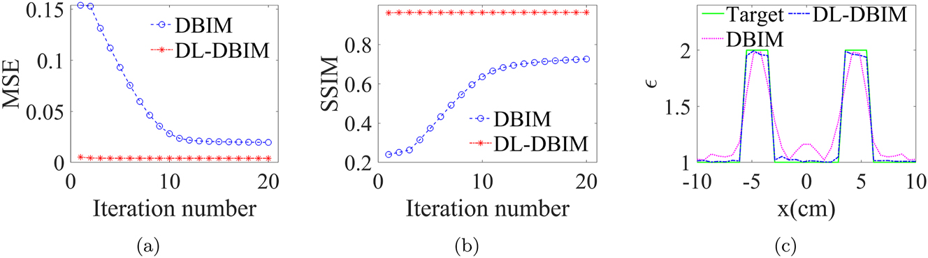
Results for homogeneous Austria profile (ϵ _r = 2), (a) MSE, (b) SSIM, (c) 1D plot along x-axis (y = 0).

Table 1:

MSE and SSIM for different scatterers.

Reference profile	Evaluation measures	DBIM		DL-DBIM
		After 5th iteration	After 20th iteration	After 5th iteration	After 20th iteration
Austria ϵ r = 2	MSE	0.0931	0.0194	0.0039	0.0039
	SSIM	0.3737	0.7264	0.9628	0.9634
	CT	9.9414 s		2.1186 s
Austria ϵ r = 2.4	MSE	0.2894	0.2768	0.0071	0.0069
	SSIM	0.1117	0.2390	0.9381	0.9428
	CT	21.6997 s		2.5253 s
L-shape ϵ r = 2	MSE	0.0265	0.0144	0.0045	0.0044
	SSIM	0.6175	0.7389	0.9309	0.9314
	CT	12.0515 s		2.5092 s
L-shape ϵ r = 2.4	MSE	0.1794	0.0711	0.0085	0.0082
	SSIM	0.3566	0.4563	0.9223	0.9249
	CT	21.3813 s		2.5346 s
Heterogeneous Austria	MSE	0.3152	0.3381	0.0118	0.0112
	SSIM	0.0866	0.1724	0.8867	0.9104
	CT	No convergence		2.8717 s
Multilayer object	MSE	0.2008	0.0792	0.0048	0.0046
	SSIM	0.5643	0.5075	0.8736	0.8775
	CT	22.1906 s		2.8857 s

Next, the scatterers with higher permittivity values are examined. These are spatially similar to the previous objects; however, the only difference is that they have a permittivity of 2.4. The reconstructed distributions of the contrast function are shown in Figure 3. As illustrated in Figure 3, due to higher multiple scattering effects, the DBIM technique fails to correctly reconstruct the image when the target under test has high contrast. Despite this, the proposed approach yields more precise reconstruction because the model has learned the relationship between the scattered field and the contrast function through extensive training. The iterative approach of DBIM is clearly time consuming, as shown in Table 1.

In order to demonstrate the robustness of the proposed method, the reconstruction is carried out on the noisy input data. Here, the scattered field of the homogeneous ‘L-shape’ object with a circular cylinder with permittivity 2 shown in Figure 3 is corrupted by a random noise with SNR = 5 dB, 15 dB, 25 dB, 35 dB, 45 dB, and 55 dB. The evaluation parameters MSE and SSIM for these SNR values after 20 iterations are shown in Table 2. The results indicate that the proposed method improves the reconstruction significantly over conventional algorithm even for the noisy input data. The proposed algorithm’s robustness is indicated by the fact that MSE does not vary significantly.

Table 2:

MSE and SSIM for noise contaminated homogeneous ‘L-shape object with a circular cylinder’ profile (ϵ _r = 2).

Noise level		5 dB	15 dB	25 dB	35 dB	45 dB	55 dB
MSE	DBIM	0.0655	0.0198	0.0150	0.0145	0.0144	0.0144
	DL-DBIM	0.0603	0.0096	0.0050	0.0045	0.0044	0.0044
SSIM	DBIM	0.4010	0.5702	0.6966	0.7335	0.7381	0.7387
	DL-DBIM	0.4276	0.6713	0.8603	0.9258	0.9318	0.9315

3.1.2 Tests on heterogeneous scatterers

Because the network is trained using homogeneous scatterers, it’s possible that the proposed technique won’t produce reliable results for objects where the contrast varies inside the same object. The first profile is spatially identical to the Austria profile, but the permittivity value of the ring, left disc, and right disc is 2.5, 2.2, and 2.8, respectively. Another example is a two-layer circular non-concentric cylinder with inner and outer radii of 2 and 6 cm, respectively. Furthermore, the inner and outer cylinders have permittivity values of 2.4 and 1.7, respectively, and are centered at (2, 0) cm and (0, 0) cm. A multilayer target configuration is sufficiently complex to provide a good test for numerical algorithms [2].

Figure 3 shows the final reconstructed outputs using the DBIM and the DL-DBIM techniques. The results clearly shows that conventional DBIM results are far from satisfactory. Despite the fact that the DL-DBIM was not trained on heterogeneous objects, its use results in a highly accurate reconstruction, giving it a high degree of generality. The main reason for this outcome is that, although the training is done on homogeneous objects, such objects include multiple scattering interfaces. Table 1 lists the MSE and SSIM values for this scenario. It shows that the proposed technique requires a longer time to converge. Nonetheless, it is significantly faster than the standard DBIM technique. It is only around the fourth iteration that it approaches convergence, which takes approximately 2.8 s. In addition, the values of evaluation measures indicate that the proposed methodology can effectively reconstruct the scatterers.

3.2 Experimental data results

To investigate the generalizability of the proposed algorithm, we consider the experimental data with real noise. This scattered field database is provided by the Institute of Fresnel [18]. The experimental test setup consists of 8 transmitters and 241 receivers. The transmitting and receiving antennas were placed 1.67 m apart from the center of the imaging domain.

In this section, a “FoamDielExt” profile is examined. As illustrated in Figure 5(a), the imaging profile comprises of a fixed foam cylinder and a plastic cylinder situated outside the foam. In this profile, the red cylinder is a plastic (ϵ _r = 3 ± 0.3), and the blue cylinder is a foam (ϵ _r  = 1.45 ± 0.15), with diameters of 3.1 cm and 8 cm, respectively. Figure 5(b) and (c) shows the imaging results for this example. The experimental data results further justify our conclusion that the DL-DBIM can produce better reconstruction than the standard DBIM. In addition, the MSE values for DBIM and DL-DBIM are 0.0341 and 0.024, respectively. As a result, the error has been reduced by a total of 29.62 %.

Figure 5:

Test results for experimental data, (a) original “FoamDielExt” profile, (b) reconstruction using DBIM, (c) reconstruction using DL-DBIM.

4 Conclusions

In this paper, the use of deep learning as initial guess solution for distorted Born iterative method (DBIM) is proposed. Iterative techniques with regularizations are frequently used to address the nonlinear inverse scattering problems. They are, however, coupled with a high computational cost and, as a result, are typically time-consuming. Also, for these methods the initial guess is critical to avoid local minimums. To overcome these challenges, we embed a deep learning-based method to the DBIM. The U-Net based convolutional neural network is used in this work, which is trained by using MNIST digits, characters, and circular objects. Various numerical examples are studied to test the efficiency of this algorithm, which includes different target configurations, namely homogeneous and heterogeneous dielectric objects. The quality of the reconstructed image is measured using the mean squared error (MSE), structural similarity index measure (SSIM) and convergence time (CT) values. The results revealed that the proposed deep learning-based method outperforms the standard DBIM technique in terms of image quality and convergence rate.

The main motivation for using 2D formulation in this work is that the inverse mathematical formulation becomes simpler with a less computational burden. However, the discussions and conclusions derived from this case can be applied to the 3D case without any restrictions. Therefore, this approach can be expanded to the case of 3D in the future.

References

[1] N. Nikolova, Introduction to Microwave Imaging, United Kingdom, Cambridge University Press, 2017.10.1017/9781316084267Search in Google Scholar
[2] M. Pastorino, Microwave Imaging, Hoboken, NJ, John Wiley & Sons, 2010.Search in Google Scholar
[3] X. Chen, Computational Methods for Electromagnetic Inverse Scattering, Singapore, Wiley-IEEE press, 2018.10.1002/9781119311997Search in Google Scholar
[4] P. M. Berg and R. E. Kleinman, “A contrast source inversion method,” Inverse Probl., vol. 13, pp. 1607–1620, 1997, https://doi.org/10.1088/0266-5611/13/6/013.Search in Google Scholar
[5] W. Chew and Y. Wang, “Reconstruction of two-dimensional permittivity distribution using the distorted Born iterative method,” IEEE Trans. Med. Imaging, vol. 9, pp. 218–225, 1990, https://doi.org/10.1109/42.56334.Search in Google Scholar PubMed
[6] X. Ye and X. Chen, “Subspace-based distorted-born iterative method for solving inverse scattering problems,” IEEE Trans. Antennas Propag., vol. 65, pp. 7224–7232, 2017, https://doi.org/10.1109/tap.2017.2766658.Search in Google Scholar
[7] X. Chen, Z. Wei, M. Li, and P. Rocca, “A review of deep learning approaches for inverse scattering problems,” Prog. Electromagn. Res., vol. 167, pp. 67–81, 2020, https://doi.org/10.2528/pier20030705.Search in Google Scholar
[8] Z. Wei and X. Chen, “Deep-learning schemes for full-wave nonlinear inverse scattering problems,” IEEE Trans. Geosci. Remote Sens., vol. 57, pp. 1849–1860, 2019, https://doi.org/10.1109/tgrs.2018.2869221.Search in Google Scholar
[9] L. Li, L. G. Wang, F. L. Teixeira, C. Liu, A. Nehorai, and T. J. Cui, “DeepNIS: deep neural network for nonlinear electromagnetic inverse scattering,” IEEE Trans. Antennas Propag., vol. 67, pp. 1819–1825, 2019, https://doi.org/10.1109/tap.2018.2885437.Search in Google Scholar
[10] Y. Sanghvi, Y. Kalepu, and U. Khankhoje, “Embedding deep learning in inverse scattering problems,” IEEE Trans. Comput. Imaging, vol. 6, pp. 46–56, 2020, https://doi.org/10.1109/tci.2019.2915580.Search in Google Scholar
[11] A. Lucas, M. Iliadis, R. Molina, and A. K. Katsaggelos, “Using deep neural networks for inverse problems in imaging: beyond analytical methods,” IEEE Signal Process. Mag., vol. 35, pp. 20–36, 2018, https://doi.org/10.1109/msp.2017.2760358.Search in Google Scholar
[12] H. M. Yao, W. E. I. Sha, and L. Jiang, “Two-step enhanced deep learning approach for electromagnetic inverse scattering problems,” IEEE Antennas Wirel. Propag. Lett., vol. 18, pp. 2254–2258, 2019, https://doi.org/10.1109/lawp.2019.2925578.Search in Google Scholar
[13] L. Li, L. G. Wang, and F. L. Teixeira, “Performance analysis and dynamic evolution of deep convolutional neural network for electromagnetic inverse scattering,” IEEE Antennas Wirel. Propag. Lett., vol. 18, pp. 2259–2263, 2019, https://doi.org/10.1109/lawp.2019.2927543.Search in Google Scholar
[14] J. Fajardo, J. Galvn, F. Vericat, C. Manuel Carlevaro, and R. M. Irastorza, “Phaseless microwave imaging of dielectric cylinders: an artificial neural networks-based approach,” Prog. Electromagn. Res., vol. 166, pp. 95–105, 2019, https://doi.org/10.2528/pier19080610.Search in Google Scholar
[15] Y. Sun, Z. Xia, and U. S. Kamilov, “Efficient and accurate inversion of multiple scattering with deep learning,” Opt. Express, vol. 26, pp. 14678–14688, 2018, https://doi.org/10.1364/oe.26.014678.Search in Google Scholar
[16] T. Anjit, R. Benny, P. Cherian, and P. Mythili, “Non-iterative microwave imaging solutions for inverse problems using deep learning,” Prog. Electromagn. Res. M, vol. 102, pp. 53–63, 2021, https://doi.org/10.2528/pierm21021304.Search in Google Scholar
[17] O. Ronneberger, P. Fischer, and T. Brox, “U-net: convolutional networks for biomedical image segmentation,” LNCS, vol. 9351, pp. 234–241, 2015.10.1007/978-3-319-24574-4_28Search in Google Scholar
[18] Geffrin, J., Sabouroux, P., and Eyraud, C., “Free space experimental scattering database continuation: experimental set-up and measurement precision,” Inverse Probl., vol. 21, pp. 117–130, 2005. https://doi.org/10.1088/0266-5611/21/6/s09.Search in Google Scholar
[19] Y. LeCun, L. Bottou, Y. Bengio, and P. Haffner, “Gradient-based learning applied to document recognition,” Proc. IEEE, vol. 86, pp. 2278–2324, 1998, https://doi.org/10.1109/5.726791.Search in Google Scholar
[20] A. D. Magdum, M. Erramshetty, and R. P. K. Jagannath, “An exponential filtering based inversion method for microwave imaging,” Radioengineering, vol. 30, pp. 496–503, 2021, https://doi.org/10.13164/re.2021.0496.Search in Google Scholar
© 2023 Walter de Gruyter GmbH, Berlin/Boston
Articles in the same Issue
- Frontmatter
- Research Articles