The One-Parameter Odd Lindley Exponential Model: Mathematical Properties and Applications

1 Introduction

Among the parametric distributions, the exponential distribution is perhaps the most widely applied statistical model in several fields. One of the reasons for its importance is that the exponential model has constant failure rate function. Additionally, this model was the first lifetime model for which statistical methods were extensively developed in the lite testing literature. The exponential distribution is used for the waiting time until the first event in a random process where events are occurring at a given rate. It is a relatively simple distribution; a random variable having this distribution is necessarily positive, and it is one of the more important distributions among those used for positive random variables. The probability density function (PDF) and the cumulative distribution function (CDF) of a random variable X with exponential distribution are

respectively, where λ>0 and x>0. The moments, the moment generating function (mgf) and several other properties of this distribution can be expressed in terms of elementary functions; see, for example, [25, Chapter 19], [12] and [30, Chapter 8].

In this paper, an alternative distribution with one parameter of exponential (Exp) distribution is presented on the basis of the odd Lindley-G (OL-G) family of distributions which was introduced in [40] with one positive scale parameter a. In this article we consider the special case OL-G with scale parameter a=1. Then the PDF and CDF of the OL-G family of distribution are reduced to

and

respectively. To this end, we use equations (1.1), (1.2) and (1.3) to obtain the so-called Type II Odd Lindley Exponential model (TIIOLExp) PDF (for x≥0)

The corresponding CDF of (1.1) is given by

and the hazard rate function (HRF) is given by

The quantile function of the TIIOLExp distribution is given as follows: if U has a uniform random number on U⁢(0,1), then

has random number on the TIIOLExp distribution, where W-1 denotes the negative branch of the Lambert W-function. We note that the Lambert W-function is defined as W⁢(z)⁢exp⁡[W⁢(z)]=z. The Lambert W-function has two real branches. The lower branch, W-1, is defined in the interval [-exp⁡(-1),1] and the upper branch, W0, is defined in the interval [-exp⁡(-1),∞] (see [40]). Also, the random number from the TIIOLExp distribution can be obtained with the solution of its CDF inverse.

The TIIOLExp density function can be expressed as an infinite mixture of exponentiated-exponential (Exp-Exp) density functions

where

and

represents the Exp-Exp density with power parameter γ>0. The CDF of the new model can be given by integrating (1.4) as

where

is the CDF of the Exp-Exp model with power parameter γ. The properties of the Exp-Exp distribution have been studied by many authors. The original paper [19] provided expressions for the survival function, the hazard rate function, the shapes of the PDF and the hazard rate function, stochastic orders, the moment generating function, moments, L-moments, the mean, the variance, the distribution of a sum of random variables following the Exp-Exp model, the distribution of extreme values, the maximum likelihood estimation including the case of censoring, the Fisher information matrix and tests of hypotheses. Since this seminal paper many authors have derived other properties, see [20, 21, 22, 36, 35, 47, 48, 39, 41, 26, 37, 1, 28, 11, 27].

Many extensions for the Exp model can be cited, such as the two-sided generalized Exp model by Korkmaz and Genç [27], the transmuted exponentiated generalized Exp model by Yousof, Afify, Alizadeh, Butt, Hamedani and Ali [42], the Kumaraswamy transmuted exponentiated Exp model by Nofal, Afify, Yousof, Granzotto and Louzada [34], the transmuted geometric Exp model by Afify, Alizadeh, Yousof, Aryal and Ahmad [2], the Kumaraswamy transmuted Exp model by Afify, Cordeiro, Yousof, Alzaatreh and Nofal [4], the complementary geometric transmuted Exp model by Afify, Cordeiro, Nadarajah, Yousof, Ozel, Nofal and Altun [3], the beta transmuted Exp model by Afify, Yousof and Nadarajah [5], the transmuted Weibull Exp model by Alizadeh, Rasekhi, Yousof and Hamedani [6], the complementary generalized transmuted Poisson Exp model by Alizadeh, Yousof, Afify, Cordeiro and Mansoor [7], the exponentiated transmuted Exp model by Merovci, Alizadeh, Yousof and Hamedani [31], the Burr X Exp model by Yousof, Afify, Hamedani and Aryal [44], the Topp–Leone generated Exp model by Aryal, Ortega, Hamedani and Yousof [9], the exponentiated generalized-Exp Poisson model by Aryal and Yousof [10], the Type I general exponential Exp model by Hamedani, Yousof, Rasekhi, Alizadeh and Najibi [23], the generalized transmuted Exp model by Nofal, Afify, Yousof and Cordeiro [33], the exponentiated Weibull Exp model by Cordeiro, Afify, Yousof, Pescim and Aryal [15], the Burr XII Exp model by Cordeiro, Yousof, Ramires and Ortega [16], the Weibull generalized Exp model by Yousof, Majumder, Jahanshahi, Ali and Hamedani [45], the beta Weibull Exp model by Yousof, Rasekhi, Afify, Alizadeh, Ghosh and Hamedani [46] and the Topp–Leone odd log-logistic Exp model by de Brito, Cordeiro, Yousof, Alizadeh and Silva [17], among others.

Let Y be a lifetime random variable having the Exp distribution G⁢(x;λ) in (1.1). The odds ratio that an individual (or component) following the lifetime Y will die (failure) at time x is [exp⁡(λ⁢x)-1]. Consider that the variability of this odds of death is represented by the random variable X and assume that it follows the Lindley model with scale =1. We can write

which is given by (1.5).

The paper is outlined as follows. In Section 2, some shapes for the TIIOLExp model are provided. In Section 3, we derive some mathematical properties of the new distribution. In Section 4, the model parameter is estimated by using the maximum likelihood (ML) method. A real data application is given in Section 5 to illustrate the flexibility of the TIIOLExp model. We assess the performance of the maximum likelihood estimators in terms of biases and mean squared errors by means of a simulation study in Section 6. Finally, some concluding remarks are presented in Section 7.

2 Shapes

For the PDF of the TIIOLExp distribution, the first and the second derivatives of f⁢(x;λ) are

Let x∗ be the critical point of ∂⁡f⁢(x;λ)∂⁡x. Then its solution is x∗=λ-1⁢log⁡2. We obtain ∂2⁡f⁢(x;λ)∂⁡x2|x=x∗<0. Hence, it has a local maximum point and the TIIOLExp distribution is unimodal. Also, for x<x∗ the PDF is increasing, and for x>x∗ the PDF is decreasing. The mode of the distribution is given by x∗. We note that limx→0⁡f⁢(x;λ)=λ2 and limx→∞⁡f⁢(x;λ)=0.

For the HRF of the TIIOLExp distribution, the first derivative of h⁢(x;λ) is

It follows that the TIIOLExp distribution has increasing HRF. We also note that limx→0⁡h⁢(x;λ)=λ2 and limx→∞⁡h⁢(x;λ)=∞. We sketched the PDF and HRF of the TIIOLExp distribution in Figure 1 for selected parameter values. These figures are consistent with the above expressions.

Figure 1

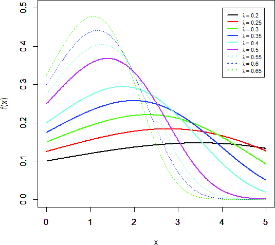
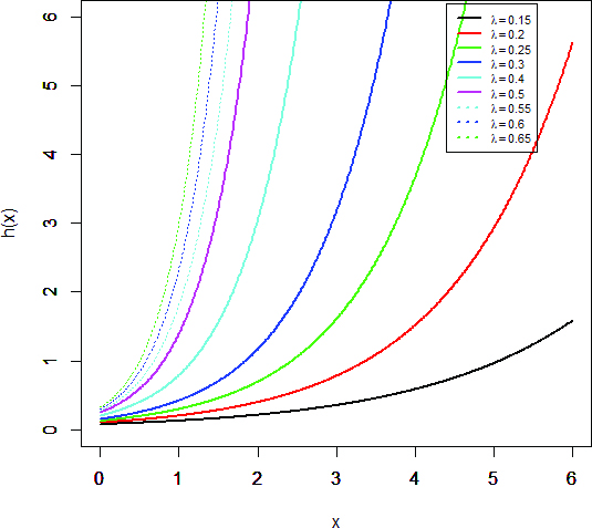
Plots of the TIIOLExp PDF and HRF for some parameter values.

3 Some Mathematical Properties

The rth moment of the TIIOLE model can be written as

where

and

The rth incomplete moment of X, say Ir⁢(t), is given by

Using equation (1.6), we obtain

where

is the incomplete gamma function. The first incomplete moment of X, denoted by I1⁢(t), is simply determined from (3.1) by setting r=1. The first incomplete moment has important applications related to the Bonferroni and Lorenz curves and the mean residual life and the mean waiting time.

The nth moment of the residual life, say zn⁢(t)=E⁢[(X-t)n⁢∣X>⁢t], n=1,2,…, uniquely determines F⁢(x). The nth moment of the residual life of X is given by

Therefore,

where

The mean residual life (MRL) function or the life expectation at age t is defined by

which represents the expected additional life length for a unit which is alive at age t. The MRL of X can be obtained by setting n=1 in the last equation. The nth moment of the reversed residual life, say Zn(t)=E[(t-X)n∣X≤t], for t>0 and n=1,2,…, uniquely determines F⁢(x). We obtain

Then the nth moment of the reversed residual life of X becomes

where

The mean inactivity time (MIT), also called the mean reversed residual life function, is given by

and it represents the waiting time elapsed since the failure of an item on condition that this failure had occurred in (0,t).

Let X1,…,Xn be a random sample from the TIIOLExp model of distributions and let X1:n,…,Xn:n be the corresponding order statistics. The PDF of the ith order statistic, say Xi:n, can be expressed as

where B⁢(⋅,⋅) is the beta function. Substituting (1.1) and (1.2) into (3.2), we obtain

where

Then the qth moment of Xi:n is given by

where

4 Estimation

Given a random sample X1,X2,…,Xn of size n from the TIIOLExp distribution with the PDF (1.4), the log-likelihood function is given by

The ML estimate λ^ of λ is the solution of the non-linear equation

where x¯ is the sample mean. To obtain the MLE of λ, we can maximize (4.1) directly with respect to λ or we can solve the non-linear equation (4.2). Note that ML estimate of the λ cannot be solved analytically; numerical iteration techniques, such as the Newton–Raphson algorithm, are adopted to solve the log-likelihood equation for which (4.1) is maximized.

The TIIOLExp distribution satisfies all the regularity conditions (see [24, Chapter 6]. Therefore applying the usual large sample approximation, the estimators λ^ are treated as being approximately normal with mean λ and variance I-1, where I is the Fisher information which is given by

Using Maple, the integral in (4.3) is obtained as

where γ is Euler’s constant which is approximately 0.5772156649⁢… and Fqp⁢([n],[d],Δ) is the generalized hypergeometric function. This function is also known as Barnes’s extended hypergeometric function. The definition of Fqp⁢([n],[d],Δ) is given by

where n=[n1,n2,…,np], p is the number of operands of n, d=[d1,d2,…,dq], q is the number of operands of d and Γ⁢(⋅) is the gamma function. The generalized hypergeometric function is quickly evaluated and readily available in standard software, such as Maple and Mathematica. Now, the asymptotic 100⁢(1-α)% confidence interval for λ^ is given by

where zα/2 is the quantile with 1-α2 of the standard normal distribution.

5 Real Data Modeling

In this section, we provide an application to see the data modeling ability of the TIIOLExp model. For the TIIOLExp model, we analyzed the stress-rupture life of kevlar 49/epoxy strands which were subjected to constant sustained pressure at the 70 % stress level until all had failed. This data set was studied by Barlow, Toland and Freeman [13], Andrews and Herzberg [8] and Cooray and Ananda [14]. The failure times in hours are 1051, 1337, 1389, 1921, 1942, 2322, 3629, 4006, 4012, 4063, 4921, 5445, 5620, 5817, 5905, 5956, 6068, 6121, 6473, 7501, 7886, 8108, 8546, 8666, 8831, 9106, 9711, 9806, 10205, 10396, 10861, 11026, 11214, 11362, 11604, 11608, 11745, 11762,11895, 12044, 13520, 13670, 14110, 14496, 15395, 16179, 17092, 17568, 17568. Using this data set, we fit the TIIOLExp, the exponential (E), the Lindley (L) (Lindley [29]), the generalized exponential (GE) (Gupta and Kundu [19]), the Nadarajah and Haghighi exponential (NH) (Nadarajah and Haghighi [32]), the extended exponential (EE) (Gomez, Bolfarine and Gomez [18]) and the Xgamma (XG) (Sen, Maiti and Chandra [38]) distribution models. The CDFs of the GE, NH, L, EE and XG models are respectively (for x>0,α,λ>0)

We compare the TIIOLExp model with the above models under the estimated log-likelihood (ℓ^) value, the Kolmogorov–Smirnov (K-S) statistics, the Akaike information criteria (AIC), the consistent Akaike information criteria (CAIC), the Bayesian information criteria (BIC) and the Hannan–Quinn information criteria (HQIC). Note that AIC, CAIC, BIC and HQIC are by given by

where p is the number of the estimated model parameters and n is the sample size. The distribution with the smallest AIC, CAIC, BIC, HQIC and K-S values and the biggest log-likelihood and p values of the K-S statistics is chosen as the best model. All calculations are obtained by maxLik routine in the R programme.

The results of this application are listed in Table 1. These results show that the TIIOLExp distribution has the lowest AIC, CAIC, BIC, HQIC and K-S values and has the biggest estimated log-likelihood and p-value of the K-S statistics among all the fitted models. So it could be chosen as the best model under these criteria. The estimated CDFs of the application models are displayed in Figure 2. It is clear from this figure that the TIIOLExp model provides the best fit to this data set as compared to other models. The 95 % confidence interval for the TIIOLExp parameter λ is then computed as [6.6620×10-6,0.00011].

Figure 2

Fitted CDFs on emprical CDF.

6 Simulation Study

In this section, we perform the simulation study using the TIIOLExp distribution. To see the performance of MLEs of this distribution, we generate 1,000 samples of sizes 20, 50 and 100 from TIIOLExp using the inverse of its CDF. We also compute the biases and mean squared errors (MSE) of the MLEs with

and

respectively. To get the inverse of the CDF, we use the uniroot routine in the R programme for random generation and use the optim routine for MLEs. The results of the simulation are reported in Table 2. From this table, we observe that when the sample size increases, the empirical mean, the standard deviations (SD), the biases and the MSEs decrease in all the cases, as expected. We also note that the SDs, biases and MSEs increase when λ increases.

7 Conclusions

In this article, an exponential model with only one shape parameter, which can be used in modeling survival data, reliability problems and fatigue life studies, was studied. We derived explicit expressions for some of its statistical and mathematical quantities including the ordinary moments, the generating function, incomplete moments, order statistics, the moment of residual life and reversed residual life. The model parameter was estimated by using the maximum likelihood method. A real data application was given to illustrate the flexibility of the model. We assessed the performance of the maximum likelihood estimators in terms of biases and mean squared errors by means of a simulation study. We hope that the new distribution will attract wider applications in engineering, reliability and other areas of research. Estimation of the TIIOLExp model parameters under the Bayesian paradigm is currently underway and will be reported in a separate article elsewhere. However, we must make a note of the fact that under the Bayesian setting, a non-informative prior approach is essentially the maximum likelihood estimation under the classical approach. In the absence of an appropriate conjugate prior, the choice of prior will be a challenge in such a setting. As a future work we will consider the bivariate and multivariate extensions of the TIIOLExp distribution, in particular with the copula based construction method, the trivariate reduction, etc.

References

[1] A. H. Abdel-Hamid and E. K. Al-Hussaini, Estimation in step-stress accelerated life tests for the exponentiated exponential distribution with type-I censoring, Comput. Statist. Data Anal. 53 (2009), no. 4, 1328–1338. 10.1016/j.csda.2008.11.006Search in Google Scholar
[2] A. Z. Afify, M. Alizadeh, H. M. Yousof, G. Aryal and M. Ahmad, The transmuted geometric-G family of distributions: Theory and applications, Pakistan J. Statist. 32 (2016), no. 2, 139–160. Search in Google Scholar
[3] A. Z. Afify, G. M. Cordeiro, S. Nadarajah, H. M. Yousof, G. Ozel, Z. M. Nofal and E. Altun, The complementary geometric transmuted-G family of distributions: Model, properties and applications, Hacet. J. Math. Stat. (2017), 10.15672/HJMS.2017.439. 10.15672/HJMS.2017.439Search in Google Scholar
[4] A. Z. Afify, G. M. Cordeiro, H. M. Yousof, Z. M. Nofal and A. Alzaatreh, The Kumaraswamy transmuted-G family of distributions: Properties and applications, J. Data Sci. 14 (2016), no. 2, 245–270. 10.6339/JDS.201604_14(2).0004Search in Google Scholar
[5] A. Z. Afify, H. M. Yousof and S. Nadarajah, The beta transmuted-H family for lifetime data, Stat. Interface 10 (2017), no. 3, 505–520. 10.4310/SII.2017.v10.n3.a13Search in Google Scholar
[6] M. Alizadeh, M. Rasekhi, H. M. Yousof and G. G. Hamedani, The transmuted Weibull G family of distributions, Hacet. J. Math. Stat. (2017), 10.15672/HJMS.2017.440. 10.15672/HJMS.2017.440Search in Google Scholar
[7] M. Alizadeh, H. M. Yousof, A. Z. Afify, G. M. Cordeiro and M. Mansoor, The complementary generalized transmuted Poisson-G family, Austrian J. Stat., to appear. 10.17713/ajs.v47i4.577Search in Google Scholar
[8] D. F. Andrews and A. M. Herzberg, Data. A Collection of Problems from Many Fields for the Student and Research Worker, Springer Ser. Statist., Springer, New York, 1985. Search in Google Scholar
[9] G. R. Aryal, E. M. Ortega, G. G. Hamedani and H. M. Yousof, The Topp Leone generated Weibull distribution: Regression model, characterizations and applications, Int. J. Statist. Probab. 6 (2017), 126–141. 10.5539/ijsp.v6n1p126Search in Google Scholar
[10] G. R. Aryal and H. M. Yousof, The exponentiated generalized-G Poisson family of distributions, Stochastics Quality Control (2017), 10.1515/eqc-2017-0004. 10.1515/eqc-2017-0004Search in Google Scholar
[11] M. Aslam, D. Kundu and M. Ahmad, Time truncated acceptance sampling plans for generalized exponential distribution, J. Appl. Stat. 37 (2010), no. 3-4, 555–566. 10.1080/02664760902769787Search in Google Scholar
[12] N. Balakrishnan and A. P. Basu, The Exponential Distribution, Gordon and Breach Publishers, Amsterdam, 1995. Search in Google Scholar
[13] R. E. Barlow, R. H. Toland and T. Freeman, A Bayesian analysis of stress-rupture life of kevlar 49/epoxy spherical pressure vessels, Proceedings of the Canadian Conference in Application Statistics, Marcel Dekker, New York (1984). Search in Google Scholar
[14] K. Cooray and M. M. A. Ananda, A generalization of the half-normal distribution with applications to lifetime data, Comm. Statist. Theory Methods 37 (2008), no. 8–10, 1323–1337. 10.1080/03610920701826088Search in Google Scholar
[15] G. M. Cordeiro, A. Z. Afify, H. M. Yousof, R. R. Pescim and G. R. Aryal, The exponentiated Weibull-H family of distributions: Theory and Applications, Mediterr. J. Math., to appear. 10.1007/s00009-017-0955-1Search in Google Scholar
[16] G. M. Cordeiro, H. M. Yousof, T. G. Ramires and E. M. M. Ortega, The Burr XII system of densities: Properties, regression model and applications, J. Stat. Comput. Simul., to appear. 10.1080/00949655.2017.1392524Search in Google Scholar
[17] E. de Brito, G. M. Cordeiro, H. M. Yousof, M. Alizadeh and G. O. Silva, Topp–Leone odd log-logistic family of distributions, J. Stat. Comput. Simul., to appear. 10.1080/00949655.2017.1351972Search in Google Scholar
[18] Y. M. Gómez, H. Bolfarine and H. W. Gómez, A new extension of the exponential distribution, Rev. Colombiana Estadíst. 37 (2014), no. 1, 25–34. 10.15446/rce.v37n1.44355Search in Google Scholar
[19] R. D. Gupta and D. Kundu, Generalized exponential distributions, Aust. N. Z. J. Stat. 41 (1999), no. 2, 173–188. 10.1111/1467-842X.00072Search in Google Scholar
[20] R. D. Gupta and D. Kundu, Exponentiated exponential family: An alternative to gamma and Weibull distributions, Biom. J. 43 (2001), no. 1, 117–130. 10.1002/1521-4036(200102)43:1<117::AID-BIMJ117>3.0.CO;2-RSearch in Google Scholar
[21] R. D. Gupta and D. Kundu, Generalized exponential distribution: different method of estimations, J. Statist. Comput. Simulation 69 (2001), no. 4, 315–337. 10.1080/00949650108812098Search in Google Scholar
[22] R. D. Gupta and D. Kundu, Generalized exponential distribution: existing results and some recent developments, J. Statist. Plann. Inference 137 (2007), no. 11, 3537–3547. 10.1016/j.jspi.2007.03.030Search in Google Scholar
[23] G. G. Hamedani, H. M. Yousof, M. Rasekhi, M. Alizadeh and S. M. Najibi, Type I general exponential class of distributions, Int. J. Appl. Exp. Math., to appear. 10.18187/pjsor.v14i1.2193Search in Google Scholar
[24] R. V. Hogg, J. W. McKean and A. T. Craig, Introduction to Mathematical Statistics, 6th ed., Pearson Education, Upper Saddle River, 2005. Search in Google Scholar
[25] N. L. Johnson, S. Kotz and N. Balakrishnan, Continuous Univariate Distributions. Vol. 1, 2nd ed., Wiley Series in Probability and Mathematical Statistics: Applied Probability and Statistics, John Wiley & Sons, New York, 1994. Search in Google Scholar
[26] C. S. Kakade and D. T. Shirke, Tolerance interval for exponentiated exponential distribution based on grouped data, Int. J. Agric. Stat. Sci. 3 (2007), 625–631. Search in Google Scholar
[27] M. C. Korkmaz and A. I. Genç, Two-sided generalized exponential distribution, Comm. Statist. Theory Methods 44 (2015), no. 23, 5049–5070. 10.1080/03610926.2013.813041Search in Google Scholar
[28] D. Kundu and B. Pradhan, Bayesian inference and life testing plans for generalized exponential distribution, Sci. China Ser. A 52 (2009), no. 6, 1373–1388. 10.1007/s11425-009-0085-8Search in Google Scholar
[29] D. V. Lindley, Fiducial distributions and Bayes’ theorem, J. Roy. Statist. Soc. Ser. B 20 (1958), 102–107. 10.1111/j.2517-6161.1958.tb00278.xSearch in Google Scholar
[30] A. W. Marshall and I. Olkin, Life Distributions, Springer Ser. Statist., Springer, New York, 2007. Search in Google Scholar
[31] F. Merovci, M. Alizadeh, H. M. Yousof and G. G. Hamedani, The exponentiated transmuted-G family of distributions: Theory and applications, Comm. Statist. Theory Methods (2016), 10.1080/03610926.2016.1248782. 10.1080/03610926.2016.1248782Search in Google Scholar
[32] S. Nadarajah and F. Haghighi, An extension of the exponential distribution, Statistics 45 (2011), no. 6, 543–558. 10.1080/02331881003678678Search in Google Scholar
[33] Z. M. Nofal, A. Z. Afify, H. M. Yousof and G. M. Cordeiro, The generalized transmuted-G family of distributions, Comm. Statist. Theory Methods 46 (2017), no. 8, 4119–4136. 10.1080/03610926.2015.1078478Search in Google Scholar
[34] Z. M. Nofal, A. Z. Afify, H. M. Yousof, D. C. T. Granzotto and F. Louzada, Kumaraswamy transmuted exponentiated additive Weibull distribution, Int. J. Statist. Probab. 5 (2016), no. 2, 78–99. 10.5539/ijsp.v5n2p78Search in Google Scholar
[35] M. Z. Raqab, Inferences for generalized exponential distribution based on record statistics, J. Statist. Plann. Inference 104 (2001), 339–350. 10.1016/S0378-3758(01)00246-4Search in Google Scholar
[36] M. Z. Raqab and M. Ahsanullah, Estimation of the location and scale parameters of generalized exponential distribution based on order statistics, J. Statist. Comput. Simulation 69 (2001), no. 2, 109–123. 10.1080/00949650108812085Search in Google Scholar
[37] A. M. Sarhan, Analysis of incomplete, censored data in competing risks models with generalized exponential distributions, IEEE Trans. Reliab. 56 (2007), 132–138. 10.1109/TR.2006.890899Search in Google Scholar
[38] S. Sen, S. S. Maiti and N. Chandra, The Xgamma distribution: statistical properties and application, J. Mod. Appl. Statist. Methods 15 (2016), 774–788. 10.22237/jmasm/1462077420Search in Google Scholar
[39] D. T. Shirke, R. R. Kumbhar and D. Kundu, Tolerance intervals for exponentiated scale family of distributions, J. Appl. Stat. 32 (2005), no. 10, 1067–1074. 10.1080/02664760500165297Search in Google Scholar
[40] F. S. G. Silva, A. Percontini, E. de Brito, M. W. Ramos, R. Venancio and G. M. Cordeiro, The odd Lindley-G family of distributions, Austrian J. Stat. 46 (2017), no. 1, 65–87. 10.17713/ajs.v46i1.222Search in Google Scholar
[41] H. M. Srivastava, S. Nadarajah and S. Kotz, Some generalizations of the Laplace distribution, Appl. Math. Comput. 182 (2006), 223–231.10.1016/j.amc.2006.01.091Search in Google Scholar
[42] H. M. Yousof, A. Z. Afify, M. Alizadeh, N. S. Butt, G. G. Hamedani and M. M. Ali, The transmuted exponentiated generalized-G family of distributions, Pak. J. Stat. Oper. Res. 11 (2015), no. 4, 441–464. 10.18187/pjsor.v11i4.1164Search in Google Scholar
[43] H. M. Yousof, A. Z. Afify, G. M. Cordeiro, A. Alzaatreh and M. Ahsanullah, A new four-parameter Weibull model for lifetime data, J. Stat. Theory Appl., to appear. Search in Google Scholar
[44] H. M. Yousof, A. Z. Afify, G. G. Hamedani and G. Aryal, The Burr X generator of distributions for lifetime data, J. Statist. Theory Appl., to appear. 10.2991/jsta.2017.16.3.2Search in Google Scholar
[45] H. M. Yousof, M. Majumder, S. M. A. Jahanshahi, M. M. Ali and G. G. Hamedani, A new Weibull class of distributions: Theory, characterizations and applications, J. Stat. Res. Iran, to appear. 10.29252/jsri.15.1.45Search in Google Scholar
[46] H. M. Yousof, M. Rasekhi, A. Z. Afify, M. Alizadeh, I. Ghosh and G. G. Hamedani, The beta Weibull-G family of distributions: Theory, characterizations and applications, Pakistan J. Statist. 33 (2017), no. 2, 95–116. Search in Google Scholar
[47] G. Zheng, On the Fisher information matrix in type II censored data from the exponentiated exponential family, Biom. J. 44 (2002), 353–357. 10.1002/1521-4036(200204)44:3<353::AID-BIMJ353>3.0.CO;2-7Search in Google Scholar
[48] G. Zheng and S. Park, A note on time savings in censored life testing, J. Statist. Plann. Inference 124 (2004), no. 2, 289–300. 10.1016/S0378-3758(03)00208-8Search in Google Scholar
© 2017 Walter de Gruyter GmbH, Berlin/Boston
Articles in the same Issue
- Frontmatter
- In Memoriam: Elart von Collani
- The Exponentiated Generalized-G Poisson Family of Distributions