IoT Energy Storage - A Forecast

1 Introduction

One of the challenges for long-life wireless Internet of Things (IoT) devices is that of energy supply. IoT devices, with only non-chargeable battery cells, have a limited lifetime based on the total battery energy provided, which makes the battery volume necessary. The available energy also limits the IoT performance in terms of, e.g. , the number of measurements, data analysis, and data communication. For IoT devices with an energy harvester, the situation changes. Many of the performance limitations will disappear or be greatly reduced. The design challenge turns into balancing energy harvesting and storage against the energy usage schedule. The energy cost for unit operations such as data sampling, computation and communication and the harvesting and storage capacity of different technologies then become important.

This paper discusses forecasts of IoT energy usage in relation to energy harvesting and storage while also considering aspect such as temperature and cycling degradation.

Energy harvesting technologies have improved over the last couple of decades. In particular, photo-voltaic harvesters have made significant progress. Other technologies more suitable for enclosed locations, such as those harvesting vibration and heat, are less mature. Recent reviews on these technologies are included in Shaikh and Zeadally (2016)

The alternatives for energy storage include rechar\-geable battery cells, supercapacitors, and capacitors. Here, cycling degradation and temperature place certain limits on the battery cells and supercapacitors. For battery cells, cyclic degradation phenomena will limit lifetimes. A survey provided by Hu et al. (2017) indicates a cyclic capability ranging from 200 to 12000 cycles depending on the battery technology, where there is also a trade off between self-discharge, power density, cost, etc. With respect to operating temperature ranges, both secondary cells and supercapacitors have limited high-temperature storage solutions. For temperatures above 100 ∘C, the supercapacitors currently available exhibit increased leakage that would consume a large part of the harvested power. As Shaikh et al. discuss in (2016), other storage devices apart from batteries and supercapacitors should be investigated.

For computational energy consumption, Koomey’s law Denning and Lewis (2016) predicts that power consumption per computation will be reduced and approach the Landauer limit, which is approximately 1000 times lower than today’s level Bérut et al. (2012). With the current rate of irreversible computing, thermal noise at room temperature will become a hindrance close to the year 2030 according to Frank (2002).

With respect to data sampling, the trends in energy cost for A/D conversion are nicely summarized by Murmann. The data indicate that for low-frequency A/D converters, the figure of merit (FoMS) trend increased from 162 dB to 182 dB between 2004 and 2017. A well-accepted limit on A/D conversion efficiency is derived from a class-B switched capacitor circuit, which yields a theoretical (FoMS) limit of 192 dB. This small gap between the state of the art and the theoretical limit indicates that there will not be any significant progress in the future, just a delay until designs have been commercialized.

In most cases, it is not the sampling or computation of data that is the most energy-demanding task for a wireless IoT device; rather, it is the transmission and reception of data over the wireless link. To minimize the energy cost of wireless transmissions, strategies have been developed to reduce the active time during which a sensor needs to listen and synchronize its transmission time slot to match the rest of the network Narendra, Duquennoy, and Voigt (2015). Time synchronization has dramatically reduced the energy spent on wireless communication; furthermore, transceivers have also become more efficient over time.

Based on available data for radio frequency (RF) transceivers, we present here the current trend for transceivers available on the market, showing how their energy cost to transport data has reduced over time with reference to the theoretical limits.

In this paper, the above data are combined to provide a forecast for IoT. We combine the RF chip trend with data on the energy cost for computation and data sampling and the energy storage efficiency for various storage technologies.

2 IoT Energy Usage and Storage

In this work, we assume that the power output from the EH is several times lower than the peak power used by the IoT device, which is the case for most of today’s EH-powered IoT devices: PEH<<Pmax.

We can express the IoT device’s average power consumption as

where P is power (watt) and t is time (s) for communication, computation, acquisition and sleep.

If each of the tasks in eq. (1) is considered uninterpretable, then the maximum product between power and time will determine the most energy expensive task. Therefore, assuming PEH<<Pmax, it is the energy storage that sets the limit on what types of tasks such a system can execute.

The power output from the EH then determines how often the tasks can be performed. The interval in which to perform tasks has to be set so that the average power consumption is lower than the power output from the EH: Pavg<PEH.

Before starting a task, especially an uninterpretable one, the IoT has to know that enough energy is available for the task to be completed. It has to create a dynamic schedule based on power input and communication time slots.

Below, an analysis of technology development trends together with currently known theoretical limits is used to predict a timeline for when no or only marginal improvement can be expected regarding data transport, computation, data acquisition and energy storage.

2.1 Wireless data Transport

The most power-intensive task for most of today’s wireless IoT devices is wireless communication. In general, it is energy efficient in that a packet transmission is completed without any interruptions. Internet packet sizes vary from 50–1500 depending on the application and the radio protocol used. Thus, ensuring that enough energy is available for transmitting a complete package is important.

2.1.1 RF Transceivers

For more than two decades, vendors have produced commercially available RF modules/chips that can transmit (TX) and receive (RX) digital data from one point to another. We have investigated datasheets for RF chips from various vendors and compared them over time. All chips have been compared using their highest sensitivity setting, highest data rate and a power output to the antenna of 1mW (0dBm).

In Figure 1, we summarize some of the common transceivers and compare their power consumption while receiving and transmitting data. Each transceiver’s power is registered according to the year that its first version was released.

Figure 1:

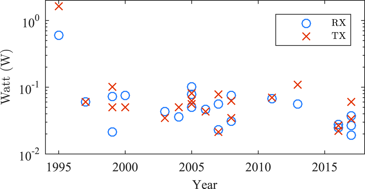
Power consumption for RF modules/chips while receiving/transmitting and when they were commercially available. RX power is taken from when the transceiver is set to its highest sensitivity state, and TX power is taken from when the transceiver outputs 1 mW (0 dbm) to the antenna.

Figure 1 does not indicate any clear trend in power reduction over time, neither in TX nor in RX.

2.1.2 Energy Per Bit

Taking data rate into consideration, one can examine how many joules per bit, Q (J/bit), is required for a full data link between two RF chips of the same kind:

(2)Q=PTX+PRXC,

where PTX (watt) is the transmitter’s power consumption, PRX (watt) is the receiver’s power consumption and C is the data rate (bit/s).

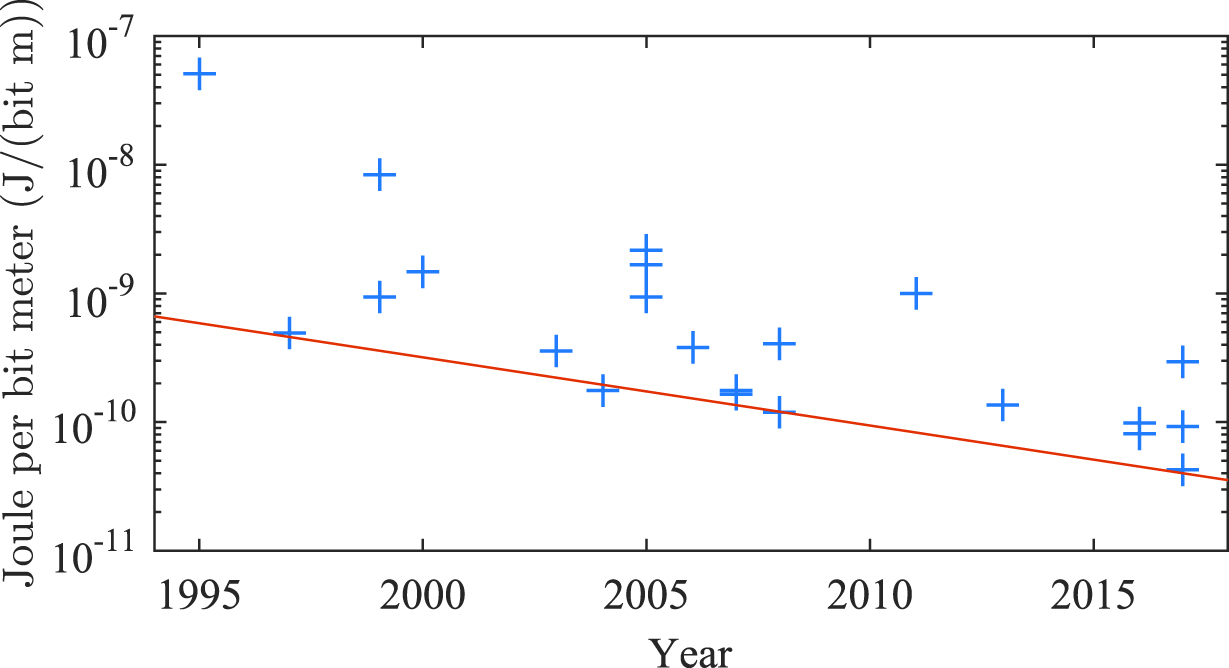
Figure 2 shows how many joules per bit is required to transmit and receive data.

Figure 2:

Energy per bit for a data link. Includes energy to both send and receive data.

From 1995 to 2007, a progress in efficiency can be observed; however, after 2007, one can not distinguish any noticeable advancements.

2.1.3 Receiver Sensitivity

Receivers have become more sensitive, meaning that the incoming signal can be weaker and the receiver can still interpret the wirelessly sent data. This advancement has made it possible to either lower the power output to reach the same distance or use the same output power to transfer data over a longer range.

To express sensitivity as the maximum distance that two transceivers can communicate with each other in free space, excluding antenna gains and noise, one can use the free space path loss

(3)FSPL(dB)=10log104πdfc2,

where d is distance in meters, f is carrier frequency in Hz and c is the speed of light. The free space path loss describes how much the signal is attenuated due to the distance between the transmitter and receiver. Hence, the requirement for two devices to communicate is dependent on having the distance between them not attenuate the signal below the sensitivity of the receiver.

The difference between the transmitter’s antenna output, Pt (watt), and the receiver’s sensitivity, Pr (watt), is called the link budget L0.

(4)L0(dB)=Pt(dB)−Pr(dB).

Hence, the required link budget L0 has to be greater than or equal to the FSPL to successfully transmit data between two devices. Substituting FSPL for L0 and solving eq. (3) for d to obtain the maximum distance two devices can communicate yields

(5)d=c10L0(dB)/104πf.

Using the data from Figure 2 and dividing it by the maximum distance, obtained by eq. (5), two transceivers of the same model can communicate with the yields shown in Figure 3. The units in Figure 3 are joules per bit and meter (J/(bit m)) or newtons per bit (N/bit). Newtons per bit can be interpreted as describing how much effort (force) an RF chip has to exert to transfer a bit a certain distance through a medium with friction. Lower values mean that the RF chip transmits and receives more efficiently.

Figure 3:

Energy per bit and meter to transfer data between two RF modules. Maximum distances between RF modules were calculated using the free space path loss eq. (5). The red line shows a trend for the top performing RF modules; it halves every sixth year.

Figure 3 shows a decreasing trend for energy spent on transmitting and receiving data a certain distance over time. The most efficient transceivers show a trend that is halved every sixth year; this trend is mostly driven by increased sensitivity and secondarily by the increased data rate.

2.1.4 RF Limitations

To address if the current trend can continue, we used Shannon-Hartley’s theorem to analyze what a theoretical limit could be. The Shannon-Hartley theorem states the maximum data capacity in the presence of noise that can be transmitted wirelessly for a given signal strength, noise and bandwidth Shannon (1949):

(6)C=Wlog2(1+PrNr),

where C is the channel capacity (bits/s), W is the bandwidth (Hz), Pr is the received signal strength (watt or volt2) and Nr is noise (watt or volt2). Solving eq. (6) for the required signal strength yields

(7)Pr=Nr(2C/W−1).

Equation (7) in eq. (4) yields the required link budget Ln in the presence of noise for a specific channel capacity and bandwidth.

(8)Ln(dB)=Pt(dB)−Nr(dB)−dB(2C/W−1)).

Figure 4:

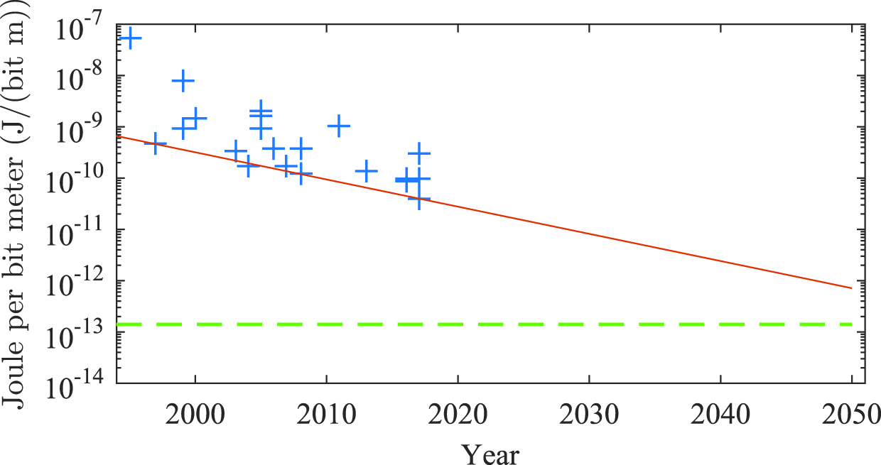
Energy per bit and meter for RF modules marked with blue markers. The red solid line shows the trend of the most efficient transceivers, and the dashed green line shows the theoretical limit for an IEEE 802.11a/g, 1 mW for TX and RX, carrier frequency 2.45 GHz, bandwidth 20 MHz, data rate 54 Mbit and noise floor -96 dBm.

Substituting the link budget, L0, for the required link budget in the presence of noise, Ln, in eq. (5) yields

(9)d=c4πf10Ln(dB)/10,

and substituting eq. (8) into eq. (9) yields

(10)d=c4πf10(Pt(dB)−Nr(dB))/102C/W−1

or

(11)d=c4πfPt(2C/W−1)Nr.

By studying eq. (11), one can observe that an increase in frequency and data rate will reduce the distance, while an increase in transmission power and bandwidth will increase the distance. However, an increase in bandwidth will also increase the received noise. Therefore, with the assumption of white noise, eq. (11) can be written as

(12)d=c4πfPt(2C/W−1)N0W,

where N0 is the noise spectral density and N0=kT, where k (J/K) is Boltzmann’s constant and T (K) is the system noise temperature.

2.1.5 Theoretical Limit

With the assumption of 100% transmission efficiency, 1 mW to the transmitter will generate 1 mW (0 dBm) of antenna output, Pt=0 dBm, and the receiver is assumed to require 1 mW to interpret the data. Using a data rate and a bandwidth of, e.g., IEEE 802.11a/g and a receiver noise floor of −96 dBm yields a theoretical limit of 1.4∗10−13 J/(bit meter). Figure 4 shows that it is likely that the trend will continue in the coming decade. However, as with the Landauer limit for computing, it will most likely never be reached, creating an asymptotic trend toward the limit according to the current knowledge.

2.2 Data Acquisition

It is common that an IoT device samples a low number of data points, e.g., a temperature measurement. Since temperature measurements are seldom performed consecutively in long high frequency series, the measurement tasks can be performed rapidly with sleeping periods in between. However, in cases where the task is to capture a waveform, it can be considered an interruptible task, where the acquisition (Pacqtacq) can be the dominating task in eq. (1). Thus, it determines the lower limit for energy storage.

Murmann et al. have summarized data for analog to digital converters (ADC) over two decades in Murmann. The data in Figure 5 indicate an increasing trend in the figure of merit (FoMS) and thus a reduction in energy per sample. For low-frequency A/D converters, the well-accepted limit of the FoMS is 192 dB, which is only 10 dB from today’s converters. Most likely, the limit of 192 dB will never be reached for room temperature devices due to the implications of thermal noise. Therefore, one cannot expect any great advancement in data acquisition with the current knowledge, just a delay until the state of the art is commercialized. Thus, this result indicates no significant advancement beyond 2025.

Figure 5:

Figure of merit for A/D converters and year of publication. The dashed green line shows the theoretical limit (192 dB) for a low speed A/D converter.

3 Analysis and Discussion

The rapid development of computing, storage and wireless communication efficiency will lead to smaller IoT devices. To show this, we have assumed a scenario of a wireless IoT device powered by a vibration harvester with a power density of 250μW/cm3Roundy, Wright, and Rabaey (2003). We assume that it receives and transmits 1 MB of data wireless 100 meters from/to another IoT device each minute. No overhead or extra time spent on listening/receiving is considered, and its sleep power is 5µW. The device uses MLCC as a storage medium. This has an evolutionary trend predicted by Pan and Randall (2010) and an RF efficiency trend shown in this paper. In the described scenario, we have assumed that it is the wireless communication that is the most energy demanding task and that it therefore determines the lower limit on the energy storage. Figure 6 shows the volume required for the device in the described scenario.

One limit on storage efficiency is discussed by Smith et al., showing that the theoretical limit on storage efficiency for glass-based ceramic capacitors is 35 J/cm3Smith et al. (2009). Assuming the same technology limit for the commercial ceramic capacitors (35 J/cm3), the limit will be reached in the year 2021 and will cap the development rate in this forecast. However, other dielectric materials can possibly achieve higher energy densities in the future. The authors have not found any evidence that 35 J/cm3 is the ultimate limit for MLCCs.

With current knowledge, noise levels will limit computational advancements close to 2030 according to Frank (2002). The limit on the RF communication efficiency calculated in this paper assumes that essentially three limits are reached. First, we assume that Shannon-Hartley’s limit is realized and we have full channel utilization. Second, sensitivity in the RF receiver is equal to the noise floor of the channel. Lastly, the RF transmitter is 100% efficient, generating 0 dBm output from 1 mW. Considering that there are three limits connected to the dashed line in Figure 4, the distance from the practical limit should be in cubic form. Therefore, we predict that the radio transceiver efficiency will level out close to the year 2035.

Figure 6:

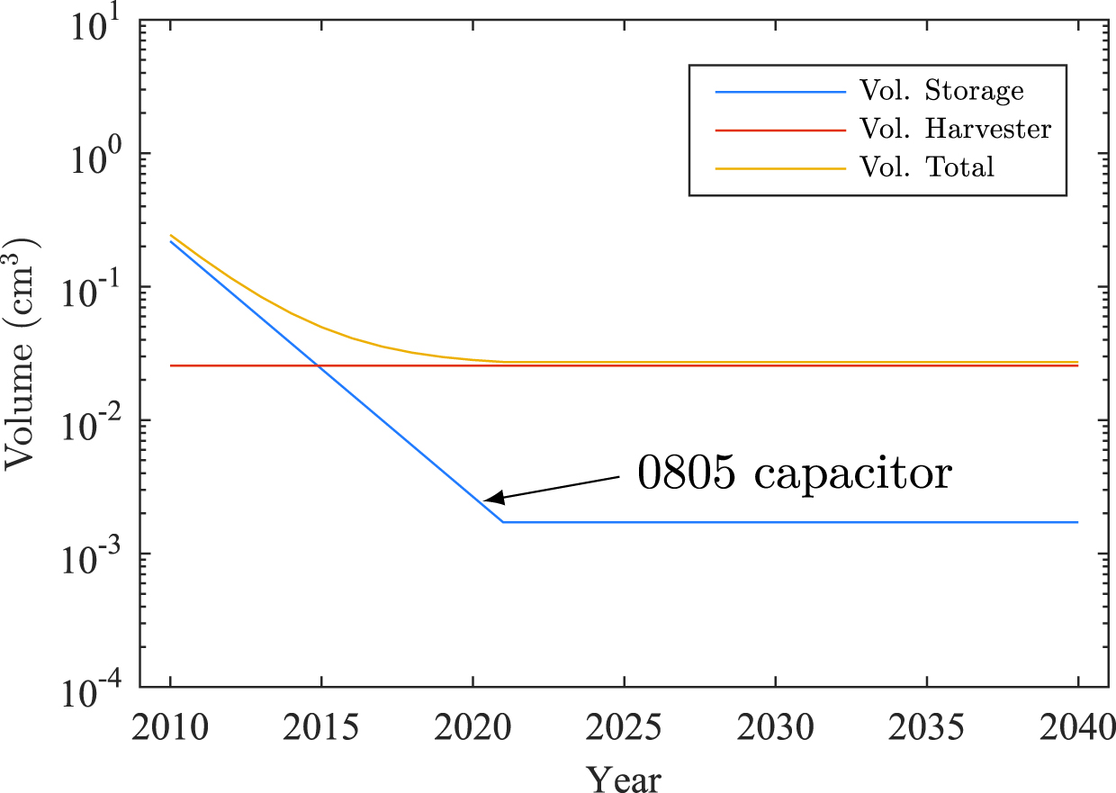
The required volume for an IoT device that receives and transmits 1 MB of data wirelessly 100 meters from/to another IoT device each minute.

The scenario above describes an ideal case, with no retransmissions, no energy spent on overhead and listening, free space path loss and no computation.

The most energy demanding task does not have to be RF communication. In Figure 7, one can observe the required volume for a system that samples continuously for 60 sec each hour with a power consumption of 1 mW. As discussed previously, A/D-conversion efficiency is close to its current known limit. Therefore, no efficiency progression in sampling is accounted for, only volumetric storage efficiency.

Figure 7:

The required volume for an IoT that samples for 60 seconds each hour.

Both Figures 6 and 7 do not account for any development in energy harvesting.

4 Conclusions

The data and trends here presented and summarized make it evident that wireless IoT devices will only use energy harvesting and short term storage such as ceramic capacitors in the future. The current development trend indicates that such wireless IoT devices are ready for today’s market. It is further clear we will not see a further reduction of energy consumption for IoT devices beyond 2035–2040.

It is expected that this type of data can enable energy modeling for large system of systems based on the IoT.

References

ARM. 2009. “ARM 180nm Ultra Low Power Platform.” http://infocenter.arm.com/help/topic/com.arm.doc.pfl0307-1/PIPD\_Platform\_TSMC\_180ULL\_BR\_NC.pdf.Search in Google Scholar
Bérut A., A. Arakelyan, A. Petrosyan, S. Ciliberto, R. Dillenschneider, and E. Lutz. 2012 “Experimental Verification of Landauer/’s Principle Linking Information and Thermodynamics.” Nature 483 (7388): 187–9.10.1038/nature10872Search in Google Scholar PubMed
Borges R. S., A. L. M. Reddy, M.-T. F. Rodrigues, H. Gullapalli, K. Balakrishnan, G. G. Silva, and P. M. Ajayan. 2013. “Supercapacitor Operating at 200 Degrees Celsius.” Scientific Reports 3.10.1038/srep02572Search in Google Scholar PubMed PubMed Central
DCN. 2017. “Super Capacitors.” http://www.illinoiscapacitor.com/ pdf/seriesDocuments/DCN%20series.pdf, 407DCN2R7Q.Search in Google Scholar
Denning P. J., and T. G. Lewis. 2016 “Exponential Laws of Computing Growth.” Communications of the ACM 60 (1): 54–65.10.1145/2976758Search in Google Scholar
El-Kady M. F., and R. B. Kaner. 2013. “Scalable Fabrication of High-Power Graphene Micro-Supercapacitors for Flexible and On-chip Energy Storage.” Nature Communications 4: 1475.10.1038/ncomms2446Search in Google Scholar PubMed
Frank M. P. 2002 “The Physical Limits of Computing.” Computing in Science & Engineering 4 (3): 16–26.10.1109/5992.998637Search in Google Scholar
Hibino T., K. Kobayashi, M. Nagao, and S. Kawasaki. 2015. “High-Temperature Supercapacitor with a Proton-Conducting metal Pyrophosphate Electrolyte.” Scientific Reports 5.10.1038/srep07903Search in Google Scholar PubMed PubMed Central
Hu X., C. Zou, C. Zhang, and Y. Li. 2017. “Technological Developments in Batteries: A Survey of Principal Roles, Types, and Management Needs.” IEEE Power and Energy Magazine 15 (5): 20–31.10.1109/MPE.2017.2708812Search in Google Scholar
Semiconductors. 2015. “International Technology Roadmap for Semiconductors (ITRS).” https://www.semiconductors. org/clientuploads/Research\_Technology/ITRS/2015/ 0\_2015%20ITRS%202.0%20Executive%20Report%20(1).pdf.Search in Google Scholar
Kim N. S., T. Austin, D. Baauw, T. Mudge, K. Flautner, J. S. Hu, M. J. Irwin, M. Kandemir, and V. Narayanan. 2003. “Leakage Current: Moore’s Law Meets Static Power.” Computer 36 (12): 68–75.10.1109/MC.2003.1250885Search in Google Scholar
Kim S.-K., H. J. Kim, J.-C. Lee, P. V. Braun, and H. S. Park. 2015. “Extremely Durable, Flexible Supercapacitors with Greatly Improved Performance at High Temperatures.” ACS Nano 9 (8): 8569–77.10.1021/acsnano.5b03732Search in Google Scholar PubMed
Kulkarni C., G. Biswas, and X. Koutsoukos. 2009. “A Prognosis Case Study for Electrolytic Capacitor Degradation in dc-dc Converters.” In PHM Conference.Search in Google Scholar
Liu C., Z. Yu, D. Neff, A. Zhamu, and B. Z. Jang. 2010. “Graphene-Based Supercapacitor with an Ultrahigh Energy Density.” Nano Letters 10 (12): 4863–8.10.1021/nl102661qSearch in Google Scholar PubMed
Merrett G. V., and A. S. Weddell. 2012. “Supercapacitor Leakage in Energy-Harvesting Sensor Nodes: Fact or Fiction?” In 2012 Ninth International Conference on Networked Sensing Systems (INSS). IEEE 2012, 1–5.10.1109/INSS.2012.6240581Search in Google Scholar
muRata. 2018. “Capacitor Data Sheet.” http://psearch.en.murata. com/capacitor/product/GRM188R6YA106MA73%23.pdf, gRM188R6YA106MA73.Search in Google Scholar
Murmann B. “Adc Performance Survey 1997-2013.” [Online]. Available: http://web.stanford.edu/murmann/adcsurvey.html.Search in Google Scholar
Narendra P., S. Duquennoy, and T. Voigt. 2015. “Ble and Ieee 802.15. 4 in the Iot: Evaluation and Interoperability Considerations.” In International Internet of Things Summit, 427–38. Springer.10.1007/978-3-319-47075-7_47Search in Google Scholar
Nichicon. 2017. “Aluminum Electrolytic Capacitors.” http://nichicon-us.com/english/products/pdfs/e-ucl.pdf, uCL1V221MCL6GS.Search in Google Scholar
Nomura T., N. Kawano, J. Yamamatsu, T. Arashi, Y. Nakano, and A. Sato. 1995. “Aging Behavior of Ni-Electrode Multilayer Ceramic Capacitors with x7r Characteristics.” Japanese Journal of Applied Physics 34 (9S): 5389.10.1143/JJAP.34.5389Search in Google Scholar
Pan M.-J., and C. A. Randall. 2010. “A Brief Introduction to Ceramic Capacitors,” IEEE Electrical Insulation Magazine 26 (3).10.1109/MEI.2010.5482787Search in Google Scholar
Roundy S., P. K. Wright, and J. Rabaey. 2003. “A Study of Low Level Vibrations as a Power Source for Wireless Sensor nodes.” Computer Communications 26 (11): 1131–44. Ubiquitous Computing. [Online]. Available: http://www.sciencedirect. com/science/article/pii/S0140366402002487.10.1016/S0140-3664(02)00248-7Search in Google Scholar
Sedlakova V., J. Sikula, J. Majzner, P. Sedlak, T. Kuparowitz, B. Buergler, and P. Vasina. 2016. “Supercapacitor Degradation Assesment by Power Cycling and Calendar Life Tests.” Metrology and Measurement Systems 23 (3): 345–58.10.1515/mms-2016-0038Search in Google Scholar
Shaikh F. K., and S. Zeadally. 2016. “Energy Harvesting in Wireless Sensor Networks: A Comprehensive Review.” Renewable and Sustainable Energy Reviews 55 (Supplement C): 1041–54. [Online]. Available: http://www.sciencedirect.com/science/ article/pii/S1364032115012629.10.1016/j.rser.2015.11.010Search in Google Scholar
Shannon C. E. 1949. “Communication in the Presence of Noise.” Proceedings of the IRE 37 (1): 10–21.10.1109/JRPROC.1949.232969Search in Google Scholar
Smith N. J., B. Rangarajan, M. T. Lanagan, and C. G. Pantano. 2009. “Alkali-Free Glass as a High Energy Density Dielectric Material.” Materials Letters 63 (15): 1245–48.10.1016/j.matlet.2009.02.047Search in Google Scholar
Tang H., and H. A. Sodano. 2013. “Ultra High Energy Density Nanocomposite Capacitors with Fast Discharge Using Ba 0.2 Sr 0.8 TiO 3 Nanowires.” Nano Letters 13 (4): 1373–9.10.1021/nl3037273Search in Google Scholar PubMed
© 2018 Walter de Gruyter Inc., Boston/Berlin
Articles in the same Issue
- Frontmatter
- Editorial
- Book Review
- Energy Harvesting – A New Publication from DEStech Publication Inc. – A Review
- Research Article