Home The (almost) integral Chow ring of ℳ̅3
Article Open Access

The (almost) integral Chow ring of ℳ̅3

  • Michele Pernice ORCID logo EMAIL logo
Published/Copyright: June 4, 2024

Abstract

This paper is the fourth in a series of four papers aiming to describe the (almost integral) Chow ring of M ̄ 3 , the moduli stack of stable curves of genus 3. In this paper, we finally compute the Chow ring of M ̄ 3 with Z [ 1 / 6 ] -coefficients.

1 Introduction

The geometry of the moduli spaces of curves has always been the subject of intensive investigations, because of its manifold implications, for instance in the study of families of curves. One of the main aspects of this investigation is the intersection theory of these spaces, which has both enumerative and geometrical implication. In his groundbreaking paper [16], Mumford introduced the intersection theory with rational coefficients for the moduli spaces of stable curves. He also computed the Chow ring (with rational coefficients) of M ̄ 2 , the moduli space of stable genus 2 curves. While the rational Chow ring of M g , the moduli space of smooth curves, is known for 2 g 9 ([16, 12, 14, 17, 3]), the computations in the stable case are much harder. The complete description of the rational Chow ring has been obtained only for genus 2 by Mumford and for genus 3 by Faber in [12]. In his PhD thesis, Faber also computed the rational Chow ring of M ̄ 2 , 1 , the moduli space of 1-pointed stable curves of genus 2.

Edidin and Graham introduced in [9] the intersection theory of global quotient stacks with integer coefficients. It is a more refined invariant, but as expected, the computations for the Chow ring with integral coefficients of the moduli stack of curves are much harder than the ones with rational coefficients. To date, the only complete description for the integral Chow ring of the moduli stack of stable curves is the case of M ̄ 2 , obtained by Larson in [15] and subsequently with a different strategy by Di Lorenzo and Vistoli in [6]. It is also worth mentioning the result of Di Lorenzo, Pernice and Vistoli regarding the integral Chow ring of M ̄ 2 , 1 ; see [5].

The aim of this series of papers is to describe the Chow ring with Z [ 1 / 6 ] -coefficients of the moduli stack M ̄ 3 of stable genus 3 curves. This provides a refinement of the result of Faber with a completely independent method. The approach is a generalization of the one used in [5]: we introduce an Artin stack, which is called the stack of A r -stable curves, where we allow curves with A r -singularities to appear. The idea is to compute the Chow ring of this newly introduced stack in the genus 3 case and then, using localization sequence, find a description for the Chow ring of M ̄ 3 . The stack M ̃ g , n of stable A 2 -curves introduced in [5] is contained as an open substack inside our stack. We state the main theorem.

Theorem 1.1

Let 𝜅 be a base field of characteristic different from 2 , 3 , 5 , 7 . The Chow ring of M ̄ 3 with Z [ 1 / 6 ] -coefficients is the quotient of the graded polynomial algebra

Z [ 1 / 6 , λ 1 , λ 2 , λ 3 , δ 1 , δ 1 , 1 , δ 1 , 1 , 1 , H ] ,

where

  • λ 1 , λ 2 , λ 3 are the lambda classes,

  • δ 1 (respectively δ 1 , 1 , δ 1 , 1 , 1 ) is the fundamental class of the locus with one (respectively two, three) separating nodes,

  • 𝐻 is the fundamental class of the hyperelliptic locus.

The quotient ideal is generated by 15 homogeneous relations, where
  • 1 of them is in codimension 2,

  • 5 of them are in codimension 3,

  • 8 of them are in codimension 4,

  • 1 of them is in codimension 5.

At the end of this paper, we explain how to compare the result of Faber with ours and comment about the information we lose in the process of tensoring with rational coefficients.

Stable A r -curves and the strategy of the proof

The strategy for the computation is the same as that used in [5] for the integral Chow ring of M ̄ 2 , 1 . Suppose we have a closed immersion of smooth stacks Z X and we know how to compute the Chow rings of 𝒵 and X Z . We would like to use the well-known localization sequence

CH ( Z ) CH ( X ) CH ( X Z ) 0

to get the complete description of the Chow ring of 𝒳. To this end, we make use of a patching technique which is at the heart of the Borel–Atiyah–Seigel–Quillen localization theorem, and it has been used by many authors in the study of equivariant cohomology, equivariant Chow ring and equivariant K-theory. See the introduction of [6] for a more detailed discussion.

In general, without information regarding the kernel of the pushforward of the closed immersion Z X , there is no hope to get the complete description of the Chow ring of 𝒳. However, if the top Chern class of the normal bundle N Z | X is a non-zero divisor inside the Chow ring of 𝒵, we can recover CH ( X ) from CH ( X Z ) , CH ( Z ) and some patching information. We will refer to the condition on the top Chern class of the normal bundle as the gluing condition. The gluing condition implies that the troublesome kernel is trivial. See Lemma 2.12 for a more detailed statement.

Unfortunately, there is no hope that this condition is verified if 𝒵 is a Deligne–Mumford separated stack, because in this hypothesis the integral Chow ring is torsion above the dimension of the stack. This follows from [9, Theorem 3.2]. This is exactly the reason that motivated the authors of [5] to introduce the stack of cuspidal stable curves, which is not a Deligne–Mumford separated stack because it has some positive-dimensional affine stabilizers. However, introducing cusps is not enough in the case of M ̄ 3 to have the gluing condition verified (for the stratification we choose). This motivated us to introduce a generalization of the moduli stack of cuspidal stable curves, allowing curves with A r -singular points to appear in our stack. They are a natural generalization of nodes and cusps, and étale locally are plane singularities described by the equation y 2 = x r + 1 .

Future prospects

As pointed out in the introduction of [5], the limitations of this strategy are not clear. It seems that the more singularities we add, the more it is likely that the gluing condition is verified. However, adding more singularities implies that we have to eventually compute the relations coming from such loci, which can be hard. Moreover, we are left with a difficult problem, namely to find the right stratification for these newly introduced stacks. We hope that this strategy will be useful to study the intersection theory of M ̄ 3 , 1 or M ̄ 4 . Moreover, we believe that our approach can be used to obtain a complete description for the integral Chow ring of M ̄ 3 . We have not verified the gluing condition with integer coefficients because we do not know the integral Chow ring of some of the strata. However, one can try to prove alternative descriptions for these strata, for instance using weighted blowups, and compute their integral Chow ring using these descriptions. See [13] for an example.

Outline of the paper

This is the fourth (and last) paper in the series. It focuses on computing the Chow ring of the moduli stack of stable curves of genus 3.

Specifically, Section 2 is dedicated to recalling the theory of A r -stable curves as discussed in [20], the theory of hyperelliptic A r -stable curves as in [18] and the setting introduced in [19] for the computation of the Chow ring of M ̃ 3 7 . In particular, we state again the main results needed for this paper, such as the existence of the contraction morphism, the description of the hyperelliptic locus and the description of the Chow ring of M ̃ 3 7 . In the last part of the section, we discuss the strategy adopted for the computation of the Chow ring of M ̄ 3 from the Chow ring of M ̃ 3 7 . Specifically, we introduce a stratification of the closed complement of M ̄ 3 inside M ̃ 3 7 and explain why it suffices to study the locally closed strata of the stratification and their Chow rings.

In Section 3, we find a list of generators for the ideal of relation coming from the closed complement of M ̄ 3 inside M ̃ 3 7 . We prove in fact that such ideal is generated only by the fundamental class of the locally closed strata introduced in Section 2, plus some cycles coming from the open stratum.

In Section 4, we explicitly compute the relations using the gluing lemma, restricting the fundamental classes of the locally closed strata to the stratification used in [19] to compute the Chow ring of M ̃ 3 7 . This is the most difficult part of the paper in terms of computations and it uses a lot of results and notation from [19].

Finally, we summarize the results in the main theorem in Section 5, where we discuss the connection between our description and Faber’s one of the rational Chow ring of M ̄ 3 .

2 Preliminaries and strategy

In this section, we recall the definition of the moduli stack M ̃ g , n r parametrizing 𝑛-pointed A r -stable curves of genus 𝑔 and some results regarding this moduli stack. For a more detailed treatment of the subject, see [20]. Furthermore, we recall the definition of the moduli stack H ̃ g r parametrizing hyperelliptic A r -stable curves of genus 𝑔 and the alternative description using the theory of cyclic covers. For a more detailed treatment of the subject, see [18]. Moreover, we recall the strategy used for the computation of the (almost) integral Chow ring of M ̃ 3 7 , in particular stating the gluing lemma (see Lemma 2.12) and describing the stratification we used. For a more detailed treatment of the subject, see [19]. Finally, we explain how to obtain the description of the (almost) integral Chow ring of M ̄ 3 from the one of M ̃ 3 7 .

Moduli stack of A r -stable curves

Fix a non-negative integer 𝑟. Let 𝑔 be an integer with g 2 and let 𝑛 be a non-negative integer.

Definition 2.1

Let 𝑘 be an algebraically closed field and C / k a proper reduced connected one-dimensional scheme over 𝑘. We say the 𝐶 is a A r -prestable curve if it has at most A r -singularity, i.e. for every p C ( k ) , we have an isomorphism

O ̂ C , p k [ [ x , y ] ] / ( y 2 x h + 1 )

with 0 h r . Furthermore, we say that 𝐶 is A r -stable if it is A r -prestable and the dualizing sheaf ω C is ample. An 𝑛-pointed A r -stable curve over 𝑘 is an A r -prestable curve together with 𝑛 smooth distinct closed points p 1 , , p n such that ω C ( p 1 + + p n ) is ample.

Remark 2.2

Notice that an A r -prestable curve is l.c.i. by definition; therefore, the dualizing complex is in fact a line bundle.

We fix a base field 𝜅 where all the primes smaller than r + 1 are invertible. Every time we talk about genus, we intend arithmetic genus, unless specified otherwise. We recall a useful fact.

Remark 2.3

Let 𝐶 be a connected, reduced, one-dimensional, proper scheme over an algebraically closed field. Let 𝑝 be a rational point which is a singularity of A r -type. We denote by b : C ̃ C the partial normalization at the point 𝑝 and by J b the conductor ideal of 𝑏. Then a straightforward computation shows that

  1. if r = 2 h , then g ( C ) = g ( C ̃ ) + h ;

  2. if r = 2 h + 1 and C ̃ is connected, then g ( C ) = g ( C ̃ ) + h + 1 ,

  3. if r = 2 h + 1 and C ̃ is not connected, then g ( C ) = g ( C ̃ ) + h .

If C ̃ is not connected, we say that 𝑝 is a separating point. Furthermore, the Noether formula gives us that b ω C ω C ̃ ( J b ) .

We can define M ̃ g , n r as the fibered category over 𝜅-schemes whose objects are the data of A r -stable curves over 𝑆 with 𝑛 distinct sections p 1 , , p n such that every geometric fiber over 𝑆 is an 𝑛-pointed A r -stable curve. These families are called 𝑛-pointed A r -stable curves over 𝑆. Morphisms are just morphisms of 𝑛-pointed curves.

We recall the following description of M ̃ g , n r . See [20, Theorem 2.2] for the proof of the result.

Theorem 2.4

M ̃ g , n r is a smooth connected algebraic stack of finite type over 𝜅. Furthermore, it is a quotient stack: that is, there exists a smooth quasi-projective scheme X with an action of GL N for some positive 𝑁 such that M ̃ g , n r [ X / GL N ] .

Remark 2.5

Recall that we have an open embedding M ̃ g , n r M ̃ g , n s for every r s . Notice that M ̃ g , n r = M ̃ g , n 2 g + 1 for every r 2 g + 1 .

The usual definition of the Hodge bundle extends to our setting. See [20, Proposition 2.4] for the proof. As a consequence, we obtain a locally free sheaf H g of rank 𝑔 on M ̃ g , n r , which is called the Hodge bundle.

Furthermore, we recall the existence of the (minimal) contraction morphism. This is [20, Theorem 2.5].

Theorem 2.6

We have a morphism of algebraic stacks

γ : M ̃ g , n + 1 r C ̃ g , n r ,

where C ̃ g , n r is the universal curve of M ̃ g , n r . Furthermore, it is an open immersion and its image is the open locus C ̃ g , n r , 2 in C ̃ g , n r parametrizing 𝑛-pointed A r -stable curves ( C , p 1 , , p n ) of genus 𝑔 and a (not necessarily smooth) section 𝑞 such that 𝑞 is an A h -singularity for h 2 .

The hyperelliptic locus

We recall the definition of hyperelliptic A r -stable curves.

Definition 2.7

Let 𝐶 be an A r -stable curve of genus 𝑔 over an algebraically closed field. We say that 𝐶 is hyperelliptic if there exists an involution 𝜎 of 𝐶 such that the fixed locus of 𝜎 is finite and the geometric categorical quotient, which is denoted by 𝑍, is a reduced connected nodal curve of genus 0. We call the pair ( C , σ ) a hyperelliptic A r -stable curve and such 𝜎 is called a hyperelliptic involution.

We define H ̃ g r as the following fibered category: its objects are the data of a pair ( C / S , σ ) where C / S is an A r -stable curve over 𝑆 and 𝜎 is an involution of 𝐶 over 𝑆 such that ( C s , σ s ) is an A r -stable hyperelliptic curve of genus 𝑔 for every geometric point s S . These are called hyperelliptic A r -stable curves over 𝑆. A morphism is a morphism of A r -stable curves that commutes with the involutions.

Now we introduce another description of H ̃ g r , useful for understanding the link with the smooth case, using cyclic covers of twisted curves. We refer to [1] for the theory of twisted nodal curves, although we consider only twisted curves with μ 2 as stabilizers and with no markings. We refer to [2] for the moduli theory of cyclic covers.

Definition 2.8

Let 𝒵 be a twisted nodal curve of genus 0 over an algebraically closed field. We denote by n Γ the number of stacky points of Γ and by m Γ the number of intersections of Γ with the rest of the curve for every irreducible component Γ of 𝒵. Let ℒ be a line bundle on 𝒵 and let i : L 2 O Z be a morphism of O Z -modules. We denote by g Γ the quantity n Γ / 2 1 deg L | Γ .

  1. We say that ( L , i ) is hyperelliptic if the following are true:

    1. the morphism Z B G m induced by ℒ is representable,

    2. i does not vanish restricted to any stacky point.

  2. We say that ( L , i ) is A r -prestable and hyperelliptic of genus 𝑔 if ( L , i ) is hyperelliptic, χ ( L ) = g and the following are true:

    1. i does not vanish restricted to any irreducible component of 𝒵 or equivalently the morphism i : L 2 O Z is injective,

    2. if 𝑝 is a non-stacky node and i vanishes at 𝑝, then r 3 and the vanishing locus V ( i ) p of i localized at 𝑝 is a Cartier divisor of length 2,

    3. if 𝑝 is a smooth point and i vanishes at 𝑝, then the vanishing locus V ( i ) p of i localized at 𝑝 has length at most r + 1 .

  3. We say that ( L , i ) is A r -stable and hyperelliptic of genus 𝑔 if it is A r -prestable and hyperelliptic of genus 𝑔 and the following are true for every irreducible component Γ in 𝒵:

    1. if g Γ = 0 , then we have 2 m Γ n Γ 3 ,

    2. if g Γ = 1 , then we have m Γ 3 ( n Γ = 0 ).

Remark 2.9

The conditions listed above may be interpreted as properties of the induced cyclic cover C Z . Namely, conditions (a) imply that 𝐶 is a 𝐶 is a scheme, thus a curve; conditions (b) imply that 𝐶 is an A r -prestable curve; conditions (c) imply that 𝐶 is in fact A r -stable.

Let us define now the stack classifying these data. We denote by C ( 2 , g , r ) the fibered category defined in the following way: the objects are triplets ( Z S , L , i ) , where Z S is a family of twisted curves of genus 0, ℒ is a line bundle on 𝒵 and i : L 2 O Z is a morphism of O Z -modules such that the restrictions ( L s , i s ) to the geometric fibers over 𝑆 are A r -stable and hyperelliptic of genus 𝑔. Morphisms are defined as in [2].

We recall the following result, which gives us an alternative description of H ̃ g r . See [18, Propositions 2.14 and 2.21] for the proof of the result.

Proposition 2.10

The fibered category C ( 2 , g , r ) is isomorphic to H ̃ g r .

Finally, we recall the following theorem which is a consequence of [18, Proposition 2.23 and Section 3].

Proposition 2.11

The moduli stack H ̃ g r of A r -stable hyperelliptic curves of genus 𝑔 is smooth and the open H g parametrizing smooth hyperelliptic curves is dense in H ̃ g r . In particular, H ̃ g r is connected. Moreover, the natural morphism H ̃ g r M ̃ g r defined by the association ( C , σ ) C is a closed embedding between smooth algebraic stacks.

The Chow ring of M ̃ 3 7

In this subsection, we describe briefly the strategy used for the computation of the Chow ring of M ̃ 3 7 . Every Chow ring is considered with Z [ 1 / 6 ] -coefficients unless otherwise stated. Recall that our base field 𝜅 has characteristic different from 2 , 3 , 5 , 7 .

First of all, we recall the gluing lemma. Let i : Z X be a closed immersion of smooth global quotient stacks over 𝜅 of codimension 𝑑 and let U : = X Z be the open complement and j : U X the open immersion. It is straightforward to see that the pullback morphism i : CH ( X ) CH ( Z ) induces a morphism CH ( U ) CH ( Z ) / ( c d ( N Z | X ) ) , where N Z | X is the normal bundle of the closed immersion. This morphism is denoted by i by abuse of notation.

Therefore, we have the following commutative diagram of rings:

where 𝑞 is just the quotient morphism.

Lemma 2.12

In the situation above, the induced map

ζ : CH ( X ) CH ( Z ) × CH ( Z ) ( c d ( N Z | X ) ) CH ( U )

is surjective and ker ζ = i Ann ( c d ( N Z | X ) ) . In particular, if c d ( N Z | X ) is a non-zero divisor in CH ( Z ) , then 𝜁 is an isomorphism.

From now on, we refer to the condition c d ( N Z | X ) is not a zero divisor as the gluing condition.

We can apply Lemma 2.12 to the following stratification of M ̃ 3 7 :

where Δ ̃ 1 (respectively Δ ̃ 1 , 1 , Δ ̃ 1 , 1 , 1 ) is the moduli stack parametrizing A 7 -stable curves of genus 3 with a least one (respectively two, three) separating nodes. The diagram above represents the poset associated to the stratification. More precisely, our approach focuses firstly on the computation of the Chow ring of M ̃ 3 7 Δ ̃ 1 . We compute the Chow ring of H ̃ 3 7 Δ ̃ 1 ; then we apply the gluing lemma to M ̃ 3 7 ( H ̃ 3 7 Δ ̃ 1 ) and H ̃ 3 7 Δ ̃ 1 to get a description for the Chow ring of M ̃ 3 7 Δ ̃ 1 . Furthermore, we apply Lemma 2.12 to Δ ̃ 1 Δ ̃ 1 , 1 and M ̃ 3 7 Δ ̃ 1 to describe the Chow ring of M ̃ 3 7 Δ ̃ 1 , 1 , and then apply it again to M ̃ 3 7 Δ ̃ 1 , 1 and Δ ̃ 1 , 1 Δ ̃ 1 , 1 , 1 . The same procedure allows us to glue also Δ ̃ 1 , 1 , 1 and get the description of the Chow ring of M ̃ 3 7 .

Remark 2.13

Notice that we need the surjectivity of the pullback of the closed immersion to apply Lemma 2.12. For such stratification, it follows from the following results:

  • ̵‌[19, Corollaries 2.14 and 2.22] for the closed immersion i H : H ̃ 3 7 Δ ̃ 1 M ̃ 3 7 Δ ̃ 1 ;

  • [19, Propositions 4.3–4.4] for the closed immersion i 1 : Δ ̃ 1 Δ ̃ 1 , 1 M ̃ 3 7 Δ ̃ 1 , 1 ;

  • [19, Propositions 5.5–5.6] for the closed immersion i 1 , 1 : Δ ̃ 1 , 1 Δ ̃ 1 , 1 , 1 M ̃ 3 7 Δ ̃ 1 , 1 , 1 ;

  • [19, Proposition 6.2] for the closed immersion i 1 , 1 , 1 : Δ ̃ 1 , 1 , 1 M ̃ 3 7 .

For a more precise description of the strata and for the computations needed, see [19]. We recall the main theorem of [19], which describes CH ( M ̃ 3 7 ) as a Z [ 1 / 6 ] -algebra of finite presentation.

Theorem 2.14

We have the following isomorphism:

CH ( M ̃ 3 7 ) Z [ 1 / 6 ] [ λ 1 , λ 2 , λ 3 , H , δ 1 , δ 1 , 1 , δ 1 , 1 , 1 ] / I ,

where 𝐼 is generated by the following relations:

  • k h , which comes from the generator of ker i H , where i H : H ̃ 3 7 Δ ̃ 1 M ̃ 3 7 Δ ̃ 1 ;

  • k 1 ( 1 ) and k 1 ( 2 ) , which come from the two generators of ker i 1 , where

    i 1 : Δ ̃ 1 Δ ̃ 1 , 1 M ̃ 3 7 Δ ̃ 1 , 1 ;

  • k 1 , 1 ( 1 ) , k 1 , 1 ( 2 ) and k 1 , 1 ( 3 ) , which come from the three generators of ker i 1 , 1 , where

    i 1 , 1 : Δ ̃ 1 , 1 Δ ̃ 1 , 1 , 1 M ̃ 3 7 Δ ̃ 1 , 1 , 1 ;

  • k 1 , 1 , 1 ( 1 ) , k 1 , 1 , 1 ( 2 ) , k 1 , 1 , 1 ( 3 ) and k 1 , 1 , 1 ( 4 ) , which come from the four generators of ker i 1 , 1 , 1 where i 1 , 1 , 1 : Δ ̃ 1 , 1 , 1 M ̃ 3 7 ;

  • m ( 1 ) , m ( 2 ) , m ( 3 ) and 𝑟, which are the liftings of the generators of the relations of the open stratum M ̃ 3 7 ( H ̃ 3 7 Δ ̃ 1 ) ;

  • h ( 1 ) , h ( 2 ) and h ( 3 ) , which are the liftings of the generators of the relations of the stratum H ̃ 3 7 Δ ̃ 1 ;

  • d 1 ( 1 ) , which is the lifting of the generator of the relations of the stratum Δ ̃ 1 Δ ̃ 1 , 1 .

Furthermore, h ( 2 ) , h ( 3 ) and d 1 ( 1 ) are in the ideal generated by the other relations.

We have the following geometric description of the generators:

  • λ i is the 𝑖-th Chern class of the Hodge bundle H ̃ of M ̃ 3 7 for i = 1 , 2 , 3 ;

  • 𝐻 is the fundamental class of the hyperelliptic locus H ̃ 3 7 in M ̃ 3 7 ;

  • δ 1 (respectively δ 1 , 1 , δ 1 , 1 , 1 ) is the fundamental class of the closed substack Δ ̃ 1 (respectively Δ ̃ 1 , 1 , Δ ̃ 1 , 1 , 1 ).

For an explicit description of the relations, see [19, Remark 7.4].

2.1 Strategy of the computation for M ̄ 3

The final goal of this paper is to compute the Chow ring of M ̄ 3 . Since we have that M ̄ 3 is an open inside the M ̃ 3 7 , we can use the localization exact sequence

CH ( M ̃ 3 7 M ̄ 3 ) CH ( M ̃ 3 7 ) CH ( M ̄ 3 ) 0

to compute the Chow ring of M ̄ 3 as the quotient of the Chow ring of M ̃ 3 7 by the ideal generated by the image of the pushforward of the closed immersion M ̃ 3 7 M ̄ 3 M ̃ 3 7 . The paper is dedicated to computing this specific ideal.

We recall the notation used in [20, Section 4]. Let g 2 and r 1 be two integers and let 𝜅 be the base field of characteristic either 0 or greater than 2 g + 1 . We recall the sequence of open substacks (see Remark 2.5)

M ̃ g 0 M ̃ g 1 M ̃ g r

and we define A ̃ n : = M ̃ g r M ̃ g n 1 for n = 0 , , r + 1 setting M ̃ g 1 : = . By construction, M ̄ g is equal to the open M ̃ g 1 = M ̃ g r A ̃ 2 . In our setting, we need to describe the ideal generated by the image of the pushforward of the closed embedding A ̃ 2 M ̃ 3 7 .

We now introduce an alternative to A ̃ n which is easier to describe. Suppose 𝑛 is a positive integer smaller than or equal to 𝑟 and let A n be the substack of the universal curve C ̃ g r of M ̃ g r parametrizing pairs ( C / S , p ) , where 𝑝 is a section whose geometric fibers over 𝑆 are A r -singularities for r n . We give to A n the structure of closed substack of C ̃ g r inductively on 𝑛. Clearly, if n = 0 , we have

A 0 = C ̃ g r .

To define A 1 , we need to find the stack-theoretic structure of the singular locus of the natural morphism

C ̃ g r M ̃ g r .

This is standard and it can be done by taking the zero locus of the first Fitting ideal of Ω C ̃ g r | M ̃ g r . We have that A 1 M ̃ g r is now finite and it is unramified over the nodes, while it ramifies over the more complicated singularities. Therefore, we can denote by A 2 the substack of A 1 defined by the zeroth Fitting ideal of Ω A 1 | M ̃ g r . A local computation shows us that A 2 M ̃ g r is unramified over the locus of A 2 -singularities and ramified elsewhere. Inductively, we can iterate this procedure considering the zeroth Fitting ideal of Ω A n 1 | M ̃ g r to define A n .

A local computation shows that the geometric points of A n are exactly the pairs ( C , p ) such that 𝑝 is an A n -singularity for n n r .

Let us define A n : = A n A n + 1 for n = 0 , , r 1 . We have a stratification of A 2 ,

A r = A r A r 1 A 2 ,

where the A n ’s are the associated locally closed strata for n = 2 , , r .

The first reason we choose to work with A n instead of A ̃ n is the smoothness of the locally closed substack A n of C ̃ g r .

Proposition 2.15

The stack A n is smooth.

See [20, Proposition 4.1] for the proof.

The second reason is that we have an explicit description of A n that allows us to compute their Chow rings. In particular, we have the following results when 𝑛 is an even positive integer.

Proposition 2.16

A 2 m is an affine bundle of dimension m 1 over the stack M ̃ g m , [ 2 m ] r for m 1 .

The stack M ̃ g m , [ h ] r classifies A r -stable curves 𝐶 of genus g m with a smooth section 𝑞 such that ω C ( h q ) is ample. For the proof of the previous result, see [20, Corollary 4.12].

When 𝑛 is odd, things are a bit more complicated. In fact, A 2 m 1 is the disjoint union of several connected components, namely A 2 m 1 ns and A 2 m 1 i for 0 i ( g m + 1 ) / 2 . The stack A 2 m 1 ns parametrizes pairs ( C , p ) such that the partial normalization of 𝐶 at 𝑝 is connected, whereas A 2 m 1 i parametrizes pairs ( C , p ) such that the partial normalization of 𝐶 at 𝑝 is the disjoint union of two components of genus 𝑖 and g m i + 1 . For a more detailed treatment of the subject, see [20, Section 4.1].

We have the following descriptions in the odd case.

Proposition 2.17

We have a finite étale cover of degree 2,

F ns : I 2 m 1 ns A 2 m 1 ns ,

where I 2 m 1 ns is a G m U -torsor over M ̃ g m , 2 [ m ] and 𝑈 is an algebraic group whose underlying scheme is isomorphic to A m 2 .

The stack M ̃ g m , 2 [ m ] classifies A r -stable curves 𝐶 with two smooth sections q 1 , q 2 such that ω C ( m ( q 1 + q 2 ) ) is ample. For the proof of the previous result, see [20, Proposition 4.17].

A similar statement is true for the other connected components. For the proof of the following result, see [20, Proposition 4.18].

Proposition 2.18

We have a morphism

F i : I 2 m 1 i A 2 m 1 i

where I 2 m 1 i is a G m U -torsor over M ̃ i , [ m ] × M ̃ g i m + 1 , [ m ] and 𝑈 is an algebraic group whose underlying scheme is isomorphic to A m 2 . If 2 i = g m + 1 , then F i is finite étale of degree 2; otherwise, it is an isomorphism.

Finally, we explain why we can reduce to studying the stacks A n and their Chow rings. We have the following result.

Proposition 2.19

In the case of g = 3 , the functor forgetting the section gives us a natural morphism A n A ̃ n which is finite birational and it is surjective at the level of Chow groups (after inverting 6) for every n 7 .

Proof

It follows from the fact that every A r -stable curve of genus 3 has at most three singularities of type A n for n 2 . ∎

Consider now the proper morphisms

ρ n : A n M ̃ g r

and their restrictions to A n ,

ρ n : A n M ̃ g r A ̃ n + 1 ,

which are still proper; let { f i } i I n be a set of generators of CH ( A n ) as a module over CH ( M ̃ g r ) indexed by some set I n . We choose a lifting f ̃ i of every f i to the Chow group of A n for every n = 2 , , r and every i I n . We have the following result.

Lemma 2.20

In the setting above, we have that im ( ρ 2 , ) is generated by

{ ρ n , ( f ̃ i ) } 2 n r , i I n

Proof

This is a direct consequence of [4, Lemma 3.3]. ∎

The previous lemma implies that we need to focus on finding the generators of the relations coming from the strata A n for n = 2 , , 7 . Therefore, in the next section, we study the morphism ρ n and we prove that ρ n is surjective at the level of Chow rings for every n 3 . Thus im ( ρ n , ) is generated by ρ n , ( 1 ) . The same is not true for n = 2 , but we describe geometrically the generators of the image of ρ 2 , .

3 The relations from the A n -strata

In this section, we are going to describe abstractly the generators of im ( ρ 2 , ) . Lemma 2.20 assures us it is enough to find the generators of im ( ρ n , ) for all n = 2 , , 7 and then lift them to M ̃ 3 7 . Recall that the characteristic of 𝜅 is either 0 or greater than 7. For the rest of the paper, if we do not specify the value of 𝑟 for a moduli stack of A r -stable curves, it means that we are considering the biggest moduli stack we can form considering A r -singularities. Because of Remark 2.3, we have that 𝑟 is bounded from above by a function of the genus. Following this notation, M ̃ 3 is the moduli stack M ̃ 3 7 and the same is true for the hyperelliptic locus H ̃ 3 and the universal curve C ̃ 3 . However, notice that, while M ̃ 1 , 1 is equal to M ̃ 1 , 1 2 , the notation M ̃ 1 , 2 does not stand for M ̃ 1 , 2 2 but for M ̃ 1 , 2 3 as M ̃ 1 , 2 3 M ̃ 1 , 2 2 .

Before we start with the abstract computations, we need to recall some notation and results from [20, Section 3].

Notation 3.1

Denote by F m c the moduli stack parametrizing pointed curvilinear algebras, i.e. pairs ( A , p ) over an algebraically closed field 𝑘, where 𝐴 is a local Artinian algebra over 𝑘 of length 𝑚, 𝑝 is the section associated to the maximal ideal and dim k m p / m p 2 1 . Furthermore, denote by E m , d c the moduli stack parametrizing finite flat extensions ( A , p ) ( B , q ) of degree 𝑑 of pointed curvilinear algebras where ( A , p ) is in F m c (and therefore ( B , q ) is in F d m c ).

Corollary 3.5 of [20] gives us an isomorphism between F m c and the classifying stack of G m , where G m is the automorphism group of the standard curvilinear algebra k [ t ] / ( t m ) with the standard section q 0 defined by t 0 . Notice that every automorphism of the pair ( k [ t ] / ( t m ) , q 0 ) is determined by its value on 𝑡; therefore, it follows easily that G m is isomorphic to G m U , where 𝑈 is a unipotent group (whose underlying scheme is an affine space of dimension m 2 ).

Proposition 3.7 of [20] gives us a description of E m , d as a quotient stack of a scheme E m , d by the action of G m × G m d . The scheme E m , d can be described as the set of all finite flat extensions ϕ d : k [ t ] / ( t m ) k [ t ] / ( t d m ) of degree 𝑑 and the action of G m × G d m is the natural one. Again, ϕ d is determined by its value on 𝑡 and it is easy to see that ϕ d ( t ) is a polynomial of the form

a t d + b 1 t d + 1 + + b d ( m 1 ) 1 t d m 1 ,

where a 0 . It follows that E m , d is isomorphic to ( A 1 0 ) × A d ( m 1 ) 1 .

Finally, we recall that the morphism E m , d c F d m c is an affine bundle since [ E m , d / G m ] is isomorphic to an affine space V m , d of dimension ( m 1 ) ( d 1 ) described as

V m , d : = { ϕ E m , d a 0 ( ϕ ) = 1 , a k d ( ϕ ) = 0 for k = 1 , , m 2 } ,

where a l ( ϕ ) is the coefficient of t l of the polynomial ϕ ( t ) . See [20, Lemma 3.8].

Generators for the image of ρ n , if 𝑛 is even

We are going to prove that the morphism

ρ n : CH ( M ̃ 3 7 ) CH ( A n )

is surjective for n = 4 , 6 .

Proposition 3.2

The morphism ρ 6 is surjective.

Proof

We start by considering the isomorphism proved in [20, Corollary 4.12] (see Proposition 2.16) in case m = 3 and d = 2 . It follows from [20, Proposition 4.9] that

A 6 [ V 3 , 2 / G m G a ] ;

see Notation 3.1 for a description of V 3 , 2 . As a matter of fact, we proved that the commutative diagram of stacks

is cartesian. The morphism B f can be described as the morphism of classifying stacks induced by the morphism of groups schemes f : G m G a Aut ( P 1 , ) G 6 defined by the association ϕ ϕ O P 1 O P 1 / m 6 , where m is the maximal ideal of the point ∞. For the definition of G 6 , see Notation 3.1. A simple computation, using the explicit formula of the action of G 6 on V 3 , 2 , shows that A 6 [ V 3 , 2 / G m G a ] [ A 1 / G m ] , where the action of G m on A 1 has weight −3. More explicitly, if we identify O P 1 / m 6 with the algebra κ [ t ] / ( t 6 ) , an element λ A 1 is equivalent to the inclusion of algebras κ [ t ] / ( t 3 ) κ [ t ] / ( t 6 ) defined by the association t t 2 + λ t 5 .

We want to understand the pullback of the hyperelliptic locus, i.e. ρ 6 ( H ) . It is clear that the locus ρ 6 1 ( H ̃ 3 ) is the locus in [ A 1 / G m ] such that the involution t t fixes the inclusion t t 2 + λ t 5 . This implies λ = 0 and therefore ρ 6 ( H ) = 3 s , where 𝑠 is the generator of CH ( [ A 1 / G m ] ) . This implies the surjectivity. ∎

Proposition 3.3

The morphism ρ 4 is surjective.

Proof

Again, Proposition 2.16 shows that A 4 is an affine bundle over M ̃ 1 , 1 × [ A 1 / G m ] and therefore

CH ( A 4 ) Z [ 1 / 6 , u , s ] ,

where 𝑠 is the generator of the Picard group of [ A 1 / G m ] and 𝑢 is the 𝜓-class of M ̃ 1 , 1 (which is a generator of the Chow ring of M ̃ 1 , 1 ). Exactly as it happens for the pinching morphism described in [5], we have ρ 4 ( δ 1 ) = s (see [5, Lemma 5.9]). We need to compute now ρ 4 ( H ) , where 𝐻 is the fundamental class of the hyperelliptic locus inside M ̃ 3 7 . Consider now the open immersion A 4 | M ̃ 1 , 1 A 4 induced by the open immersion M ̃ 1 , 1 M ̃ 1 , 1 × [ A 1 / G m ] . We have that

CH ( A 4 | M ̃ 1 , 1 ) = Z [ 1 / 6 , u , s ] / ( s ) ;

therefore, it is enough to prove that ρ 4 ( H ) restricted to this open is of the form 2 u to have the surjectivity of ρ 4 .

We know that M ̃ 1 , 1 [ A 2 / G m ] ; therefore, it is enough to restrict to A 4 | B G m because the pullback of the closed immersion B G m M ̃ 1 , 1 is an isomorphism of Chow rings. Similarly to the proof of Proposition 3.2, a simple computation shows that A 4 | B G m is isomorphic to [ A 1 / G m ] , where G m acts with weight −2. An element in λ A 1 is equivalent to the inclusion of algebras κ [ t ] / ( t 2 ) κ [ t ] / ( t 4 ) defined by the association t t 2 + λ t 3 .

The locus H ̃ 3 coincides with the locus in [ A 1 / G m ] described by the equation λ = 0 . Therefore, ρ 4 ( H ) = 2 u and we are done. ∎

Before going to study the morphism ρ 2 , we need to understand its source. We have that

A 2 M ̃ 2 , 1 × [ A 1 / G m ] .

Recall that M ̃ 2 , 1 is an open substack of C ̃ 2 thanks to Theorem 2.6. Therefore, the Chow ring of M ̃ 2 , 1 is a quotient of the one of C ̃ 2 . Notice that, as specified at the beginning of Section 3, C ̃ 2 is the universal curve of M ̃ 2 7 = M ̃ 2 5 .

Lemma 3.4

The Chow ring of C ̃ 2 is a quotient of the polynomial ring generated by

  • the 𝜆-classes λ 1 and λ 2 of degree 1 and 2 respectively,

  • the 𝜓-class ψ 1 ,

  • two classes θ 1 and θ 2 of degree 1 and 2 respectively;

furthermore, the ideal of relations is generated by
  • λ 2 θ 2 ψ 1 ( λ 1 ψ 1 ) ,

  • θ 1 ( λ 1 + θ 1 ) ,

  • θ 2 ψ 1 ,

  • θ 2 ( λ 1 + θ 1 ψ 1 ) ,

  • a homogeneous polynomial of degree 7.

Proof

We do not describe all the computation in detail. The idea is to use the stratification introduced in [5, Section 4], i.e. Θ ̃ 2 Θ ̃ 1 C ̃ 2 , where Θ ̃ 1 is the pullback of Δ ̃ 1 through to morphism C ̃ 2 M ̃ 2 and Θ ̃ 2 is the closed substack of C ̃ 2 parametrizing pairs ( C , p ) such that 𝑝 is a separating node. We denote by θ 1 and θ 2 the fundamental classes of Θ ̃ 1 and Θ ̃ 2 . Notice that the only difference with our situation is in the open stratum C ̃ 2 Θ ̃ 1 . In fact, the authors of [5, Proposition 4.1] proved that C ̃ 2 2 Θ ̃ 1 2 [ U / B 2 ] , where 𝑈 is an open inside a B 2 -representation A ̃ ( 6 ) . The same proof generalizes in the case r = 7 (see [19, Proposition 4.1]) and it gives us that C ̃ 2 7 Θ ̃ 1 7 [ A ̃ ( 6 ) 0 / B 2 ] , and therefore the zero section in A ̃ ( 6 ) gives us a relation of degree 7. We also have the following isomorphisms:

  • Θ ̃ 1 Θ ̃ 2 ( C ̃ 1 , 1 M ̃ 1 , 1 ) × M ̃ 1 , 1 ,

  • Θ ̃ 2 Δ ̃ 1 ;

thus we have the following descriptions of the Chow rings of the strata:
  • CH ( C ̃ 2 Θ ̃ 1 ) Z [ 1 / 6 , t 0 , t 1 ] / ( f 7 ) ,

  • CH ( Θ ̃ 1 Θ ̃ 2 ) Z [ 1 / 6 , t , s ] ,

  • CH ( Θ ̃ 2 ) Z [ 1 / 6 , λ 1 , λ 2 ] ,

where f 7 is a homogeneous polynomial of degree 7. Finally, one can prove the following identities:
  • λ 1 | C ̃ 2 Θ ̃ 1 = t 0 t 1 , λ 1 | Θ ̃ 1 Θ ̃ 2 = t s ;

  • λ 2 | C ̃ 2 Θ ̃ 1 = t 0 t 1 , λ 2 | Θ ̃ 1 Θ ̃ 2 = s t ;

  • ψ 1 | C ̃ 2 Θ ̃ 1 = t 1 , ψ 1 | Θ ̃ 1 Θ ̃ 2 = t , ψ 1 | Θ ̃ 2 = 0 ;

  • θ 1 | Θ ̃ 1 Θ ̃ 2 = t + s , θ 1 | Θ ̃ 2 = λ 1 ;

  • θ 2 | Θ ̃ 2 = λ 2 .

The result follows from applying the gluing lemma. ∎

Remark 3.5

Clearly, ρ 2 cannot be surjective at the level of Chow rings, as it is not true even at the level of Picard groups. In fact, the Picard group of M ̃ 3 is an abelian free group of rank 3, while the Picard group of M ̃ 2 , 1 × [ A 1 / G m ] is an abelian free group of rank 4.

We are ready for the proposition.

Proposition 3.6

The image of the pushforward of

ρ 2 : M ̃ 2 , 1 × [ A 1 / G m ] A 2 M ̃ 3 A ̃ 3

is generated by the elements ρ 2 , ( 1 ) , ρ 2 , ( s ) and ρ 2 , ( s θ 1 ) , where 𝑠 is the generator of the Chow ring of [ A 1 / G m ] and θ 1 is the fundamental class of the locus parametrizing curves with a separating node.

Proof

For this proof, we denote by λ 1 and λ 2 the Chern classes of the Hodge bundle of M ̃ 2 , 1 , whereas the 𝑖-th Chern class of the Hodge bundle of M ̃ 3 is denoted by c i ( H ) for i = 1 , 2 , 3 .

We need to describe the pullback of the generators of the Chow ring of M ̃ 3 through ρ 2 . By construction, it is easy to see that

ρ 2 ( δ 1 ) = s + θ 1 , ρ 2 ( δ 1 , 1 ) = θ 2 + s θ 1 and ρ 2 ( δ 1 , 1 , 1 ) = s θ 2 .

Notice that ρ 2 1 ( H ̃ 3 ) is the closed substack M ̃ 2 , ω × [ A 1 / G m ] of A 2 , where M ̃ 2 , ω is the closed substack of M ̃ 2 , 1 which parametrizes pairs ( C , p ) such that 𝑝 is fixed by the (unique) involution of 𝐶. To compute its class, we need to use the stratification used in the proof of Lemma 3.4. In the open stratum M ̃ 2 , 1 Θ ̃ 1 , [19, Proposition 4.4] implies that the restriction of [ M ̃ 2 , ω ] is equal to λ 1 3 ψ 1 . In the stratum Θ ̃ 1 Θ ̃ 2 , we have that the restriction is of the form 3 ψ 1 . This implies that ρ 2 ( H ) = λ 1 3 ψ 1 θ 1 .

Finally, to compute the restriction of c i ( H ) for i = 1 , 2 , 3 , we can restrict to the closed substack M ̃ 2 , 1 × B G m M ̃ 2 , 1 × [ A 1 / G m ] as the pullback of the closed immersion is clearly an isomorphism because it is the zero section of a vector bundle. The explicit description of the isomorphism M ̃ 2 , 1 × [ A 1 / G m ] A 2 (which was constructed in [5, Section 2]) implies that the morphism ρ 2 | M ̃ 2 , 1 × B G m maps an object ( C ̃ / S , q ) to the object ( C / S , p ) in the following way: consider the projective bundle P ( N q N 0 ) over 𝑆, where N q is the normal bundle of the section 𝑞 and N 0 is the pullback to 𝑆 of the 1-dimensional representation of G m of weight 1; we have two natural sections defined by the two subbundles N q and N 0 of N q N 0 , namely ∞ and 0; the object ( C / S , p ) is defined by gluing ∞ with 𝑞, pinching in 0 and then setting p : = 0 . A computation identical to the one of [5, Proposition 5.9] implies the following formulas:

  • ρ 2 ( c 1 ( H ) ) = λ 1 + ψ 1 s ,

  • ρ 2 ( c 2 ( H ) ) = λ 2 + λ 1 ( ψ 1 s ) ,

  • ρ 2 ( c 3 ( H ) ) = λ 2 ( ψ 1 s ) .

The description of the restrictions of the generators of CH ( M ̃ 3 ) gives us that the image of ρ 2 , is the ideal generated by ρ 2 , ( s i ) for every non-negative integer 𝑖. Moreover, we have that

ρ 2 ( δ 1 , 1 , 1 ) = s θ 2 = s ( ρ 2 ( δ 1 , 1 ) s ( ρ 2 ( δ 1 ) s ) ) ,

which implies that ρ 2 , ( s i ) is in the ideal generated by ρ 2 , ( 1 ) , ρ 2 , ( s ) and ρ 2 ( s 2 ) for every i 3 . Finally, we have that s θ 1 = s ( ρ 2 ( δ 1 ) s ) ; therefore, we can use s θ 1 as a generator with ρ 2 , ( 1 ) and ρ 2 , ( s ) instead of ρ 2 , ( s 2 ) . ∎

Remark 3.7

Notice that ρ 2 , ( s ) is equal to the fundamental class of the image of the morphism M ̃ 2 , 1 × B G m Δ ̃ 1 M ̃ 3 . We denote this closed substack Δ ̃ 1 c ; it parametrizes curves 𝐶 obtained by gluing a genus 2 curve with a genus 1 cuspidal curve in a separating node.

In the same way, ρ 2 , ( s θ 1 ) is equal to the fundamental class of the image of the morphism Θ ̃ 1 × B G m Δ ̃ 1 , 1 M ̃ 3 . We denote this closed substack Δ ̃ 1 , 1 c ; it parametrizes curves 𝐶 in Δ ̃ 1 , 1 such that one of the two elliptic tails is cuspidal.

Generators for the image of ρ n , if 𝑛 is odd

Now we deal with the odd case. This is a bit more convoluted as we have several strata to deal with for every 𝑛. Let us recall the descriptions we have. See Proposition 2.17 and Proposition 2.18.

First, A 2 m 1 is the disjoint union of A 2 m 1 ns and A 2 m 1 i for 0 i ( g m + 1 ) / 2 . Because g = 3 , we have the following possibilities:

  • if m = 4 , we have only one component, namely A 7 0 ;

  • if m = 3 , we have two components, namely A 5 0 and A 5 ns ;

  • if m = 2 , we have three components, namely A 3 0 , A 3 1 and A 3 ns .

First of all, notice that A 3 0 is empty, due to the stability condition. Therefore, we need to deal with 5 components.

We start with the case m = 4 .

Proposition 3.8

The pullback of the morphism ρ 7 : A 7 0 M ̃ 3 is surjective.

Proof

The proof is similar to the one of Proposition 3.2. First of all, we describe the Chow ring of A 7 0 . We can apply Proposition 2.18 and [19, Lemma 2.5] to get that

CH ( A 7 0 ) CH ( I 7 0 ) inv ,

where the invariants are taken with respect to the action of C 2 induced by the involution defined by the association

( ( C 1 , p 1 ) , ( C 2 , p 2 ) , ϕ ) ( ( C 2 , p 2 ) , ( C 1 , p 1 ) , ϕ 1 ) .

By construction, we have that I 7 0 is the fiber product of the diagram

where the morphism 𝑓 is described in the proof of Proposition 3.2 (see also Notation 3.1). A simple computation shows that I 7 0 [ A 1 / G m G a ] , where G a acts trivially and A 1 is the G m -representation with weight 2. Furthermore, one can prove that C 2 acts trivially on G m G a and acts on A 1 by the rule λ λ . Therefore, it is clear that CH ( I 7 0 ) Z [ 1 / 6 , s ] , where 𝑠 is the generator of the Chow ring of B G m and a simple computation shows the ρ 7 ( H ) = 2 s . ∎

We now deal with the case m = 3 . We have to split it in two subcases, namely A 5 0 and A 5 ns . We denote by ρ 5 0 and ρ 5 ns the restriction of ρ 5 to the two connected components A 5 0 and A 5 ns respectively.

Proposition 3.9

The pullback of the morphism ρ 5 0 : A 5 0 M ̃ 3 is surjective.

Proof

In this case, Proposition 2.18 tells us that A 5 0 is isomorphic to I 5 0 . We have a commutative diagram

where the morphism B f : B ( G m G a ) B G 3 is the same as in Proposition 3.8, whereas we recall that g : M ̃ 1 , [ 3 ] G 3 is defined by the association ( E , e ) O E / m e 3 . Because the morphism 𝑓 is injective (and therefore B f is representable) and E 3 , 1 is a G m G a -torsor, it is easy to verify that A 5 0 M ̃ 1 , 1 × [ A 1 / G m ] . Therefore, we have an isomorphism

CH ( A 5 0 ) Z [ 1 / 6 , u , s ] ,

where 𝑢 (respectively 𝑠) is the generator of the Chow ring of M ̃ 1 , 1 (respectively [ A 1 / G m ] ). We can describe ρ 5 0 in the following way: if we have a geometric point ( E , e ) in M ̃ 1 , [ 3 ] , the image is the genus 3 curve ( C , p ) obtained by gluing the projective line P 1 to 𝐸 identifying ∞ with 𝑒 in a A 5 -singularity (using the pushout construction as in [20, Proposition 4.18]) and setting p = e . Notice that there is a unique way of creating the A 5 -singularity up to a unique isomorphism of ( P 1 , ) .

Clearly, ρ 5 0 , ( δ 1 ) = s . However, ρ 5 0 , ( H ) = 0 ; therefore, we need to understand the pullback of the Chern classes of the Hodge bundle. It is enough to prove that ρ 5 0 , ( λ 1 ) = 2 u + n s for some integer 𝑛. Therefore, we can restrict the computation to the open substack

M ̃ 1 , 1 M ̃ 1 , 1 × [ A 1 / G m ] .

Moreover, as the closed embedding B G m M ̃ 1 , 1 is a zero section of a vector bundle over B G m , it is enough to do the computation restricting everything to ι : B G m M ̃ 1 , 1 × [ A 1 / G m ] . Therefore, suppose we have an elliptic cuspidal curve ( E , e ) with 𝑒 a smooth point, the image through ρ 5 0 is a 1-pointed genus 3 curve ( C , p ) constructed gluing the projective line ( P 1 , ) and ( E , e ) (identifying 𝑒 and ∞) in an A 5 -singularity and setting p : = e . We need to understand the G m -action over the vector space H 0 ( C , ω C ) . Consider the exact sequence

0 O C O E O P 1 Q 0

and the induced long exact sequence on the global sections

0 κ κ 2 Q H 1 ( C , O C ) H 1 ( E , O E ) 0 .

We know that ι ρ 5 ( λ 1 ) = c 1 G m ( H 1 ( C , O C ) ) and c 1 G m ( H 1 ( E , O E ) ) = u . It is enough to describe c 1 G m ( Q ) . Recall that 𝑄 fits in a exact sequence of G m -representations

0 O 3 = κ [ t ] / ( t 3 ) O 3 e O 3 = κ [ t ] / ( t 3 ) 2 Q 0 ,

where as usual O 3 e (respectively O 3 ) is the quotient O E / m e 3 (respectively O P 1 / m 3 ) . First of all, notice that, by construction, O 3 e and O 3 are G m -equivariantly isomorphic. Therefore, an easy computation shows that c 1 ( Q ) = c 1 ( O 3 ) = 3 u , and thus the restriction of λ 1 to B G m is equal to 2 u . ∎

Finally, a proof similar to the one of Proposition 3.8 gives us the following result.

Proposition 3.10

The pullback of the morphism ρ 5 ns : A 5 ns M ̃ 3 is surjective.

Proof

We leave it to the reader to check the details. See also Proposition 3.12 for a similar result in the non-separating case. ∎

It remains to prove the case for m = 2 , or the strata classifying tacnodes.

Proposition 3.11

The pullback of the morphism ρ 3 1 : A 3 1 M ̃ 3 is surjective.

Proof

Thanks to Proposition 2.18, we can describe A 3 1 using a C 2 -action on I 3 1 , which is a G m -torsor over the stack M ̃ 1 , [ 2 ] × M ̃ 1 , [ 2 ] , where M ̃ 1 , [ 2 ] M ̃ 1 , 1 × [ A 1 / G m ] . In fact, [19, Lemma 2.5] implies that CH ( A 3 1 ) CH ( I 3 1 ) C 2 inv . Because the pullback of the closed immersion

M ̃ 1 , 1 × B G m M ̃ 1 , 1 × [ A 1 / G m ]

is an isomorphism at the level of Chow rings, it is enough to understand the G m -torsor when restricted to ( M ̃ 1 , 1 × B G m ) × 2 . Let us denote by t i (respectively s i ) the generator of the Chow ring of M ̃ 1 , 1 (respectively B G m ) seen as the 𝑖-th factor of the product for i = 1 , 2 . Exactly as we have done in Proposition 3.6, we can describe the objects in this product as

( ( E 1 , e 1 ) , ( P ( N e 1 N s 1 ) , 0 , ) , ( E 2 , e 2 ) , ( P ( N e 2 N s 2 ) , 0 , ) ) .

We recall that N e i is the normal bundle of the section e i and N s i is the representation of G m (whose generator is s i ) with weight 1 (for i = 1 , 2 ). By construction, the first Chern class of N e is the 𝜓-class associated to an object ( E , e ) in M ̃ 1 , 1 .

The G m -torsor comes from identifying the two tangent spaces at ∞ of the two projective bundles. A computation shows that its class (namely the first Chern class of the line bundle associated to it) in the Chow ring of the product is of the form t 1 s 1 t 2 + s 2 . Therefore, if we set b i : = t i s i for i = 1 , 2 , we have the following description of the Chow ring of I 3 1 :

CH ( I 3 1 ) Z [ 1 / 6 , t 1 , t 2 , b 1 , b 2 ] / ( b 1 b 2 ) .

Furthermore, the C 2 -action over I 3 1 translates into an action on the Chow ring defined by the association ( t 1 , t 2 , b 1 , b 2 ) ( t 2 , t 1 , b 2 , b 1 ) ; therefore, it is easy to compute the ring of invariants. We have the following result:

CH ( A 3 1 ) Z [ 1 / 6 , d 1 , d 2 , b ] ,

where d 1 : = t 1 + t 2 and d 2 : = t 1 t 2 . An easy computation shows that ρ 3 1 , ( δ 1 ) = d 1 2 b and ρ 3 1 , ( δ 1 , 1 ) = d 2 b d 1 + b 2 . Finally, a computation identical to the one in the proof of Proposition 3.9 for the 𝜆-classes shows us that ρ 3 1 , ( λ 1 ) = b d 1 . The statement follows. ∎

Finally, we arrived at the end of this sequence of abstract computations.

Proposition 3.12

The pullback of the morphism ρ 3 ns : A 3 ns M ̃ 3 is surjective.

Proof

For this proof, we denote by λ i the Chern classes of the Hodge bundle of M ̃ 1 , 2 , while the Chern classes of the Hodge bundle of M ̃ 3 is denoted by c i ( H ) . Thanks to Proposition 2.17, we have that the Chow ring of A 3 ns can be recovered by the Chow ring of the G m -torsor I 3 ns over M ̃ 1 , 2 × [ A 1 / G m ] × [ A 1 / G m ] .

First of all, we know that M ̃ 1 , 2 C ̃ 1 , 1 thanks to Theorem 2.6 and we know the Chow ring of C ̃ 1 , 1 is isomorphic to

Z [ 1 / 6 , λ 1 , μ 1 ] / ( μ 1 ( λ 1 + μ 1 ) ) ;

see [5, Proposition 3.3]. It is important to remark that μ 1 is the fundamental class of the locus in C ̃ 1 , 1 parametrizing ( E , e 1 , e 2 ) such that the two sections coincide.

We need to understand the class of the G m -torsor I 3 ns over M ̃ 1 , 2 × [ A 1 / G m ] × [ A 1 / G m ] . As usual, we reduce to the closed substack M ̃ 1 , 2 × B G m × B G m . If we denote by s 1 (respectively s 2 ) the generator of the Chow ring of the first B G m (respectively the second B G m ) in the product, we have that the same description we used in Proposition 3.11 for the G m -torsor applies here and therefore we only need to understand the description of the two 𝜓-classes in CH ( M ̃ 1 , 2 ) , namely ψ 1 and ψ 2 . We claim that ψ 1 = ψ 2 . Consider the autoequivalence M ̃ 1 , 2 M ̃ 1 , 2 , which is defined by the association ( E , e 1 , e 2 ) ( E , e 2 , e 1 ) (and therefore acts on the Chow rings sending ψ 1 in ψ 2 and vice versa). It is easy to see that is isomorphic to the identity functor because of the unicity of the involution.

This implies that the class associated to the torsor I 3 ns is of the form s 1 s 2 . Because the action of C 2 on I 3 1 translates into the involution ( λ 1 , μ 1 , s 1 , s 2 ) ( λ 1 , μ 1 , s 2 , s 1 ) of the Chow ring, we finally have

CH ( A 3 ns ) Z [ 1 / 6 , λ 1 , μ 1 , s ] / ( μ 1 ( λ 1 + μ 1 ) ) ,

where s : = s 1 = s 2 . It is easy to see that ρ 3 ns , ( δ 1 ) = μ 1 . Moreover, the same ideas for the computations of the 𝜆-classes used in Proposition 3.9 give us that ρ 3 ns , ( c 1 ( H ) ) = s . Finally, it is enough to prove that ρ 3 ns , ( H ) = 12 λ 1 modulo the ideal ( μ 1 , s ) ; therefore, we can restrict our computation to M ̃ 1 , 2 M ̃ 1 , 1 M ̃ 1 , 2 × [ A 1 / G m ] × [ A 1 / G m ] . Notice that, in this situation, the G m -torsor is trivial. Recall that we have the formula H = 9 c 1 ( H ) δ 0 3 δ 1 by [11]. Therefore, it follows that ρ 3 ns , ( H ) = δ 0 . To compute δ 0 in M ̃ 1 , 2 M ̃ 1 , 1 , we can consider the natural morphism C ̃ 1 , 1 M ̃ 1 , 1 and use the fact that δ 0 = 12 λ 1 in CH ( M ̃ 1 , 1 ) . ∎

Lemma 2.20 implies that the image of ρ 2 , in CH ( M ̃ 3 ) is generated by the following cycles:

  • the fundamental classes of Δ ̃ 1 c and Δ ̃ 1 , 1 c ;

  • the fundamental classes of the images of ρ 7 , ρ 5 0 and ρ 3 1 , which are closed inside M ̃ 3 because of [20, Lemma 4.7]; by abuse of notation, we denote these closed substacks by A 7 , A 5 0 and A 3 1 respectively;

  • the fundamental classes of the closure of the images of ρ 6 , ρ 5 ns , ρ 4 , ρ 3 ns and ρ 2 ; by abuse of notation, we denote these closed substacks as A 6 , A 5 ns , A 4 , A 3 ns and A 2 respectively.

Remark 3.13

Notice that A 6 , A 4 and A 2 are the stacks we previously denoted by A ̃ 6 , A ̃ 4 and A ̃ 2 respectively. Moreover, the stacks A 5 ns and A 3 ns are substacks of A ̃ 5 and A ̃ 3 respectively.

Corollary 3.14

The Chow ring of M ̄ 3 is the quotient of the Chow ring of M ̃ 3 by the fundamental classes of A 7 , A 6 , A 5 0 , A 5 ns , A 4 , A 3 1 , A 3 ns , A 2 , Δ ̃ 1 c and Δ ̃ 1 , 1 c .

4 Explicit description of the relations

We illustrate the strategy to compute the explicit description of the relations listed in Corollary 3.14. Suppose we want to compute the fundamental class of a closed substack 𝑋 of M ̃ 3 . First of all, we need to compute the classes of the restrictions of 𝑋 on every stratum, namely

X | M ̃ 3 ( H ̃ 3 Δ ̃ 1 ) , X | H ̃ 3 Δ ̃ 1 , X | Δ ̃ 1 Δ ̃ 1 , 1 , X | Δ ̃ 1 , 1 Δ ̃ 1 , 1 , 1 , X | Δ ̃ 1 , 1 , 1 .

Once we have the explicit descriptions, we need to patch them together. Let us show how to do it for the first two strata, i.e. M ̃ 3 ( H ̃ 3 Δ ̃ 1 ) and H ̃ 3 Δ ̃ 1 . Suppose we have the description of X q : = X | M ̃ 3 ( Δ ̃ 1 H ̃ 3 ) and of X h : = X | H ̃ 3 Δ ̃ 1 in their respective Chow rings. Then we can compute X | M ̃ 3 Δ ̃ 1 using Lemma 2.12. Suppose we are given

X | M ̃ 3 Δ ̃ 1 = p + H q CH ( M ̃ 3 Δ ̃ 1 )

an expression of 𝑋 (which makes sense because of Remark 2.13), we need to compute the two polynomials 𝑝 and 𝑞. If we restrict 𝑋 to M ̃ 3 ( H ̃ 3 Δ ̃ 1 ) , we get that the polynomial 𝑝 can be chosen to be just any lifting of X q . Now if we restrict to H ̃ 3 Δ ̃ 1 , we get that

i h p + c top ( N H | M ) i h q = X h ,

where as usual i h : H ̃ 3 Δ ̃ 1 M ̃ 3 Δ ̃ 1 is the closed immersion of the hyperelliptic stratum and N H | M is the normal bundle of this immersion. Because of the commutativity of the diagram in Lemma 2.12, we have that X h i h p is in the ideal in CH ( H ̃ 3 Δ ̃ 1 ) generated by c top ( N H | M ) . However, the top Chern class is a non-zero divisor; thus we can choose 𝑞 to be just a lifting of q ̃ , where q ̃ is an element in CH ( H ̃ 3 Δ ̃ 1 ) such that X h i h p = c top ( N H | M ) q ̃ . Although we have made a lot of choices, it is easy to see that the presentation of X | M ̃ 3 Δ ̃ 1 is unique in the Chow ring of M ̃ 3 Δ ̃ 1 , i.e. two different presentations differ by a relation in the Chow ring.

Remark 4.1

Before proceeding with the computation, we recall the description of the Chow rings of the strata.

  • The Chow ring of H ̃ 3 7 Δ ̃ 1 is a quotient of Z [ 1 / 6 , λ 1 , λ 2 , ξ 1 ] , where λ 1 , λ 2 are the lambda classes and ξ 1 is the fundamental class of the locus Ξ 1 classifying hyperelliptic curves whose quotient by the hyperelliptic involution is not smooth (see [19, Corollary 2.14]).

  • The Chow ring of Δ ̃ 1 Δ ̃ 1 , 1 M ̃ 1 , 1 × M ̃ 2 , 1 is a quotient of Z [ 1 / 6 , t 0 , t 1 , t ] , where t 0 , t 1 are the two generators of CH ( M ̃ 2 , 1 ) and 𝑡 is the generator of M ̃ 1 , 1 (see [19, Proposition 4.3]).

  • There is a C 2 -torsor

    ( M ̃ 1 , 2 M ̃ 1 , 1 ) × M ̃ 1 , 1 × M ̃ 1 , 1 Δ ̃ 1 , 1 Δ ̃ 1 , 1 , 1 ,

    which gives us that

    CH ( Δ ̃ 1 , 1 Δ ̃ 1 , 1 , 1 ) Z [ 1 / 6 , c 1 , c 2 , t ] ,

    where c 1 , c 2 are respectively the sum and the product of the generators of the Chow rings of the two copies of M ̃ 1 , 1 , while 𝑡 is the generator of CH ( M ̃ 1 , 2 M ̃ 1 , 1 ) (see [19, Proposition 5.5]).

  • There is an S 3 -torsor

    M ̃ 1 , 1 × M ̃ 1 , 1 × M ̃ 1 , 1 Δ ̃ 1 , 1 , 1 ,

    which gives us that

    CH ( Δ ̃ 1 , 1 , 1 ) Z [ 1 / 6 , c 1 , c 2 , c 3 ] ,

    where c 1 , c 2 , c 3 are the symmetric functions in the generators of the Chow rings of the three copies of M ̃ 1 , 1 (see [19, Section 6]).

For the rest of the section, we will follow the notation set in Remark 4.1 for the generators of the Chow rings of the strata.

We show how to apply this strategy firstly for the computations of the fundamental classes δ 1 c and δ 1 , 1 c of Δ ̃ 1 c and Δ ̃ 1 , 1 c respectively. For a definition of these loci, see Remark 3.7.

Proposition 4.2

We have the following description:

δ 1 c = 6 ( δ 1 ( H + λ 1 + 3 δ 1 ) 2 + 4 δ 1 , 1 ( λ 1 H 2 δ 1 ) + 12 δ 1 , 1 , 1 ) ,

and

δ 1 , 1 c = 24 ( δ 1 , 1 ( δ 1 + λ 1 ) 2 + δ 1 , 1 , 1 δ 1 )

in the Chow ring of M ̃ 3 .

Proof

First of all, we have that Δ ̃ 1 c Δ ̃ 1 ; therefore, the generic expression of the class δ 1 c is of the form δ 1 p 2 + δ 1 , 1 p 1 + δ 1 , 1 , 1 p 0 , where p 0 , p 1 , p 2 are homogeneous polynomials in Z [ 1 / 6 , λ 1 , λ 2 , λ 3 , δ 1 , δ 1 , 1 , δ 1 , 1 , 1 , H ] of degree 0 , 1 , 2 respectively. Again, this is due to the surjectivity of the pullbacks; see Remark 2.13. We start by restricting δ 1 c to M ̃ 3 Δ ̃ 1 , 1 . Here we have the sequence of embeddings

Δ ̃ 1 c ( Δ ̃ 1 Δ ̃ 1 , 1 ) ( Δ ̃ 1 Δ ̃ 1 , 1 ) M ̃ 3 Δ ̃ 1 , 1 ,

which implies that δ 1 c restricted to CH ( Δ ̃ 1 Δ ̃ 1 , 1 ) is equal 24 t 2 ( t + t 1 ) , where 24 t 2 is the fundamental class of the closed embedding Δ ̃ 1 c Δ ̃ 1 (restricted to the open Δ ̃ 1 Δ ̃ 1 , 1 ), while ( t + t 1 ) is the normal bundle of the closed embedding i 1 : Δ ̃ 1 Δ ̃ 1 , 1 M ̃ 3 Δ ̃ 1 , 1 . Because t + t 1 is not a zero divisor in the Chow ring, we have that i 1 ( p 2 ) = 24 t 2 , which implies p 2 = 6 ( H + λ 1 + 3 δ 1 ) 2 (see [19, Proposition 4.4]).

Now we have to compute the restriction of δ 1 c to Δ ̃ 1 , 1 Δ ̃ 1 , 1 , 1 . This is not trivial because Δ ̃ 1 c is contained in Δ ̃ 1 but the closed immersion

Δ ̃ 1 , 1 Δ ̃ 1 , 1 , 1 Δ ̃ 1 Δ ̃ 1 , 1 , 1

is not regular. As a matter of fact, one can prove that doing the naive computation does not work, i.e. the difference δ 1 c δ 1 p 2 restricted to Δ ̃ 1 , 1 Δ ̃ 1 , 1 , 1 is not divisible by the top Chern class of the normal bundle of i 1 , 1 : Δ ̃ 1 , 1 Δ ̃ 1 , 1 , 1 M ̃ 3 Δ ̃ 1 , 1 , 1 . To do it properly, we can consider the following cartesian diagram:

where

μ 1 : ( M ̃ 1 , 2 M ̃ 1 , 1 ) × M ̃ 1 , 1 ( Θ ̃ 1 Θ ̃ 2 ) C ̃ 2 Θ ̃ 2 M ̃ 2 , 1 Θ ̃ 2

is described in the proof of Lemma 3.4 and ρ 2 c is the restriction of ρ 2 to the closed substack Δ ̃ 1 c . Notice that μ 1 × id is a regular embedding of codimension 1, whereas i 1 , 1 is regular of codimension 2. Excess intersection theory implies that

i 1 , 1 ( δ 1 c ) = ρ 2 , c ( 1 ) = ρ 1 , 1 , ( c 1 ( ρ 1 , 1 N i 1 , 1 / N μ 1 × id ) ) ;

the normal bundle N μ 1 was described in [5, Proposition 4.9], while N i 1 , 1 was described in [19, Proposition 5.6] (see also the proof of Lemma 3.4). A computation shows that

c 1 ( ρ 1 , 1 N i 1 , 1 / N μ × id ) = ( t + t 2 ) ,

where 𝑡 is the generator of CH ( M ̃ 1 , 2 M ̃ 1 , 1 ) , while t 2 is the generator of CH ( B G m ) . Finally, we need to compute ρ 1 , 1 , ( t + t 2 ) . This can be done by noticing that ρ 1 , 1 factors through the morphism described in [19, Lemma 5.1], i.e. the diagram

is commutative, where ρ ̃ 1 , 1 is induced by the zero section

B G m [ A 2 / G m ] M ̃ 1 , 1 .

A simple computation using the fact that π 2 is a C 2 -torsor gives us

δ 1 c | Δ ̃ 1 , 1 Δ ̃ 1 , 1 , 1 = 24 ( c 1 t 2 2 c 2 t + c 1 3 3 c 1 c 2 ) .

Using the explicit description of the pullback i 1 , 1 , we can compute ( δ 1 c δ 1 p 2 ) | Δ ̃ 1 , 1 Δ ̃ 1 , 1 , 1 and verify it is divisible by c 2 + t c 1 + t 2 (which is the second Chern class of the normal bundle of i 1 , 1 ). This gives us i 1 , 1 p 1 = 24 ( 2 t 3 c 1 ) and therefore p 1 = 24 ( λ 1 H 2 δ 1 ) .

Finally, we have to restrict δ 1 c to Δ ̃ 1 , 1 , 1 . Again, we can consider the following diagram:

where the right square is cartesian, the morphism

μ 2 : Θ ̃ 2 C ̃ 2 M ̃ 2 , 1

is the closed immersion described in [5, Section 4] (see also the proof of Lemma 3.4), the morphism c 2 : M ̃ 1 , 1 × M ̃ 1 , 1 Δ ̃ 1 Θ ̃ 2 is the gluing morphism (see proof of [5, Lemma 4.8]) and c 6 is the morphism described in [19, Lemma 6.1]. Excess intersection theory implies that

δ 1 c | Δ ̃ 1 , 1 , 1 = α ( N μ 2 ) ;

moreover, we have that

N μ 2 = ( c 2 × id ) ρ ̃ 2 ( t 1 + t 2 ) 2 ,

where t i is the generator of the 𝑖-th factor of the product M ̃ 1 , 1 × 3 for i = 1 , 2 , 3 . Therefore,

δ 1 c | Δ ̃ 1 , 1 , 1 = c 6 , ( 12 t 3 2 ( t 1 + t 2 ) ) = 24 ( c 1 c 2 3 c 3 )

in the Chow ring of Δ ̃ 1 , 1 , 1 . This leads finally to the description. The same procedure can be used to compute the class of δ 1 , 1 c .

Remark 4.3

The relation δ 1 c gives us that we do not need the generator δ 1 , 1 , 1 in CH ( M ̄ 3 ) .

The fundamental class of A 5 0 and A 3 1

Now we concentrate on describing two of the strata of separating singularities, namely A 3 1 and A 5 1 . Let us start with A 3 1 .

Proposition 4.4

We have the description

[ A 3 1 ] = H 2 ( H + λ 1 + δ 1 ) ( 3 H + λ 1 + δ 1 )

in the Chow ring of M ̃ 3 .

Proof

A generic object in A 3 1 can be described as two genus 1 curves intersecting in a separating tacnode. We claim that the morphism A 3 1 M ̃ 3 (which is proper by [20, Lemma 4.7]) factors through Ξ 1 H ̃ 3 M ̃ 3 . In fact, given an element ( ( E 1 , e 1 ) , ( E 2 , e 2 ) , ϕ ) in A 3 1 with E 1 and E 2 smooth genus 1 curves, we can consider the hyperelliptic involution of E 1 (respectively E 2 ) induced by the complete linear system of O ( 2 e 1 ) (respectively O ( 2 e 2 ) ). It is easy to see that their differentials commute with the isomorphism 𝜙, and therefore we get an involution of the genus 3 curve whose quotient is a genus 0 curve with one node. Because we have considered a generic element and the hyperelliptic locus is closed, we get the claim. In particular, A 3 1 | M ̃ 3 ( H ̃ 3 Δ ̃ 1 ) is zero.

Consider now the description of H ̃ 3 Δ ̃ 1 as in [19, Section 2]. Because

A 3 1 Δ ̃ 1 Ξ 1 Δ ̃ 1 H ̃ 3 Δ ̃ 1 ,

we have that excess intersection theory gives us the equalities

[ A 3 1 ] | H ̃ 3 Δ ̃ 1 = c 1 ( N H | M ) [ a 3 ] = 2 ξ 1 λ 1 3 [ a 3 ] ,

where a 3 is the class of A 3 1 as a codimension 2 closed substack in H ̃ 3 Δ ̃ 1 . Suppose we have an element ( Z / S , L , f ) in H ̃ 3 Δ ̃ 1 ; first of all, we have that A 3 1 Ξ 1 ; therefore, Z / S is a nodal curve of genus 0 with exactly one node. Furthermore, because we have a separating tacnode between two genus 1 curves, it is clear that the nodal section 𝑛 in 𝑍 has to be in the branching locus. Due to the description of Ξ 1 , we have that

[ A 3 1 ] | H ̃ 3 Δ ̃ 1 = 1 3 a 3 ( 2 ξ 1 λ 1 ) = 2 9 ( ξ 1 + λ 1 ) ( 2 ξ 1 λ 1 ) ξ 1 .

Let us focus on the restriction to Δ ̃ 1 Δ ̃ 1 , 1 ( M ̃ 2 , 1 Θ ̃ 1 ) × M ̃ 1 , 1 . It is easy to see that the only geometric objects that are in A 3 1 are of the form ( ( C , p ) , ( E , e ) ) , where 𝑝 lies in an almost-bridge of the genus 2 curve 𝐶, i.e. 𝑝 is a smooth point in a projective line that intersects the rest of the curve in a tacnode. Recall that we have an open immersion

M ̃ 2 , 1 Θ ̃ 1 C ̃ 2 Θ ̃ 1

described in Theorem 2.6. Through this identification, ( C , p ) corresponds to a pair ( C , p ) , where C is an A r -stable genus 2 curve and p is a cuspidal point. Therefore, it is easy to see that, in the notation of [19, Corollary 4.2], we have that the fundamental class of the separating tacnodes is described by the equations s = a 5 = a 4 = 0 . We get the following expression:

[ A 3 1 ] | Δ ̃ 1 Δ ̃ 1 , 1 = 2 t 1 ( t 0 2 t 1 ) ( t 0 3 t 1 ) CH ( Δ ̃ 1 Δ ̃ 1 , 1 ) .

The same idea works for Δ ̃ 1 , 1 Δ ̃ 1 , 1 , 1 (using [19, Lemma 5.2]) and gives us the following description:

[ A 3 1 ] | Δ ̃ 1 , 1 Δ ̃ 1 , 1 , 1 = 24 t 3 CH ( Δ ̃ 1 , 1 Δ ̃ 1 , 1 , 1 ) .

Finally, it is clear that A 3 1 Δ ̃ 1 , 1 , 1 = . ∎

Now we focus on the fundamental class of A 5 0 . A generic object in A 5 0 can be described as a genus 1 curve and a genus 0 curve intersecting in an A 5 -singularity. Notice that this implies that A 5 0 H ̃ 3 = because the only possible involution of an A 5 -singularity has to exchange the two irreducible components. In the same way, it is easy to prove that A 5 0 Δ ̃ 1 , 1 = .

The intersection of A 5 0 with Δ ̃ 1 is clearly transversal; therefore,

[ A 5 0 ] | Δ ̃ 1 Δ ̃ 1 , 1 = [ A 5 0 Δ ̃ 1 ] .

Lemma 4.5

We have the equality

[ A 5 0 ] | Δ ̃ 1 Δ ̃ 1 , 1 = 72 ( t 0 + t 1 ) 3 t 0 t 1 384 ( t 0 + t 1 ) ( t 0 t 1 ) 2

in the Chow ring of Δ ̃ 1 Δ ̃ 1 , 1 .

Proof

Because every A 5 -singularity for a curve of genus 2 is separating, it is enough to compute the fundamental class of the locus of A 5 -singularities in C ̃ 2 Θ ̃ 1 . We know that

C ̃ 2 Θ ̃ 1 [ A ̃ ( 6 ) 0 / B 2 ] ;

see [19, Corollary 4.2] for a more detailed discussion. We have that an element ( f , s ) A ̃ ( 6 ) defines a genus 2 curve with an A 5 -singularity if and only if f A ( 6 ) has a root of multiplicity 6. Because B 2 is a special group, it is enough to compute the 𝑇-equivariant fundamental class of the locus parametrizing sections of A ( 6 ) which have a root of multiplicity 6, where 𝑇 is the maximal torus inside B 2 . Therefore, one can use the formula in Remark A.7. ∎

It remains to describe the restriction of A 5 0 in M ̃ 3 ( H ̃ 3 Δ ̃ 1 ) . First of all, we pass to the projective setting. Recall that

M ̃ 3 ( H ̃ 3 Δ ̃ 1 ) [ U / GL 3 ] ,

where 𝑈 is an invariant open inside a GL 3 -representation of the space of forms in three coordinates of degree 4. Because 𝑈 does not contain the zero section, we can consider the projectivization U ̄ in P 14 and we have the isomorphism CH GL 3 ( U ) CH GL 3 ( U ̄ ) / ( c 1 h ) , where c 1 is the first Chern class of the standard representation of GL 3 and ℎ is the restriction of c 1 ( O P 14 ( 1 ) ) . We want to describe the locus X 5 0 [ P 2 × P 14 / GL 3 ] which parametrizes pairs ( f , p ) such that 𝑝 is a separating A 5 -singularity of 𝑓. Because a quartic in P 2 has at most one A 5 -singularity, we can compute the pushforward through π : [ P 14 × P 2 / GL 3 ] [ P 14 / GL 3 ] of the fundamental class of X 5 0 and then set h = c 1 to the get the fundamental class of A 5 0 . Notice that every pair ( f , p ) X 5 0 can be described as a cubic 𝑔 and a line 𝑙 such that f = g l and 𝑝 is the only intersection between 𝑔 and 𝑙, or equivalently 𝑝 is a flex of 𝑔 and 𝑙 is the flex tangent.

To describe X 5 0 , we first introduce the locally closed substack X 2 of [ P 14 × P 2 / GL 3 ] which parametrizes pairs ( f , p ) such that 𝑝 is a A r -singularity of 𝑓 with r 2 (eventually r = ).

Recall that we have the isomorphism [ P 14 × P 2 / GL 3 ] [ P 14 / H ] , where 𝐻 is the stabilizer subgroup of GL 3 of the point [ 0 : 0 : 1 ] in P 2 . The isomorphism is a consequence of the transitivity of the action of GL 3 on P 2 . Moreover, we have H ( GL 2 × G m ) G a 2 ; see [19, Remark 3.13]. We set G : = ( B 2 × G m ) G a 2 , where B 2 GL 2 is the Borel subgroup of upper triangular matrices inside GL 2 .

Finally, let us denote by 𝐿 the standard representation of G m , by 𝐸 the standard representation of GL 2 and E 0 E the flag induced by the action of B 2 on 𝐸; E 1 is the quotient E / E 0 . We denote by V 3 the 𝐻-representation ( L Sym 3 E ) Sym 4 E .

Lemma 4.6

In the setting above, we have the isomorphism

X 2 [ V 3 E 0 2 L 2 / G ]

of algebraic stacks.

Proof

Thanks to the isomorphism [ P 14 × P 2 / GL 3 ] [ P 14 / H ] , we can describe X 2 as a substack of the right-hand side. The coordinates of [ P 14 / H ] are the coefficients of the generic polynomial p = a 00 + a 10 x + a 01 y + + a 04 y 4 which is the dehomogenization of the generic quartic 𝑓 vanishing at the point [ 0 : 0 : 1 ] . First of all, notice that X 2 is contained in the complement of the closed substack 𝑋 parametrizing polynomials 𝑓 such that its first and second derivatives in 𝑥 and 𝑦 vanish at ( 0 , 0 ) : = [ 0 : 0 : 1 ] , thanks to [19, Lemma 3.6]. This is an 𝐻-equivariant subbundle of codimension 6 in [ P 14 / H ] defined by the equations

a 00 = a 10 = a 01 = a 20 = a 11 = a 02 = 0 .

We denote it simply by [ P 8 / H ] . Moreover, X 2 is contained in the locus parametrizing quartics 𝑓 such that 𝑓 is singular at ( 0 , 0 ) . This is an 𝐻-equivariant subbundle defined by the equations a 00 = a 10 = a 01 = 0 . We denote it simply [ P 11 / H ] ; therefore, X 2 [ P 11 P 8 / H ] . By construction, P 11 can be described as the projectivization of the 𝐻-representation 𝑉 defined as ( L 2 Sym 2 E ) V 3 , whereas P 8 is the projectivization of V 3 .

Consider an element 𝑝 in P 11 , described as the polynomial

a 20 x 2 + a 11 x y + a 02 y 2 + p 3 ( x , y ) + p 4 ( x , y ) ,

where p 3 and p 4 are homogeneous polynomials in x , y of degree 3 and 4 respectively. Notice that ( 0 , 0 ) is an A 1 -singularity, i.e. an ordinary node, if and only if a 11 2 4 a 02 a 20 0 . In fact, an 𝐴-singularity (eventually A ) is a node if and only if it has two different tangent lines. Therefore, X 2 is equal to the locus where the equality holds, and therefore it is enough to describe V ( a 11 2 4 a 02 a 20 ) in [ P 11 P 8 / H ] .

We define 𝑊 as the 𝐻-representation

W : = ( L E ) ( L Sym 3 E ) Sym 4 E

and we consider the 𝐻-equivariant closed embedding of W V induced by the morphism of 𝐻-schemes

L E Sym 2 ( L E ) L 2 Sym 2 E ,

which is defined by the association ( f 1 , f 2 ) ( f 1 2 , 2 f 1 f 2 , f 2 2 ) . Now, consider the G m -action on 𝑊 defined using weight 1 on the 2-dimensional vector space ( L E ) and weight 2 on V 3 . We denote by P 1 , 2 ( W ) the quotient stack and by P 2 ( V 3 ) P 1 , 2 ( W ) the closed substack induced by the embedding V 3 W . One can prove that the morphism

[ P 1 , 2 ( W ) P 2 ( V 3 ) / H ] [ P ( V ) P ( V 3 ) / H ]

induced by the closed immersion W V is a closed immersion too and its stack-theoretic image is exactly the locus V ( a 11 2 4 a 02 a 20 ) . We are considering the action of 𝐻 on a stack as defined in [21]. Finally, because the action of GL 2 over E is transitive, we have the isomorphism

[ P 1 , 2 ( W ) P 2 ( V 3 ) / H ] [ P 1 , 2 ( W 0 ) P 2 ( V 3 ) / G ] ,

where the 𝐺-representation W 0 W is defined as ( L E 0 ) V 3 . We want to stress that this is true only if we remove the locus P 2 ( V 3 ) ; in fact, the subgroup of stabilizers of W 0 in 𝑊 is equal to 𝐻 when restricted to V 3 . Finally, we notice that we have an 𝐻-equivariant isomorphism

P 1 , 2 ( W 0 ) P 2 ( V 3 ) V 3 ( E 0 2 L 2 )

of stacks. ∎

Remark 4.7

By construction, an element f V 3 E 0 2 L 2 is associated to the curve y 2 = f ( x , y ) . Notice that E is the vector space E 0 E 1 , where 𝑥 is a generator for E 1 and 𝑦 is a generator for E 0 . Moreover, L is generated by 𝑧, where ( x , y , z ) are a basis of the dual of the standard representation of GL 2 .

Corollary 4.8

We have an isomorphism of rings CH ( X 2 ) Z [ 1 / 6 , t 1 , t 2 , t 3 ] , where t 1 , t 2 , t 3 are the first Chern classes of the standard representations of the three copies of G m in 𝐺. Specifically, t 1 , t 2 , t 3 are the first Chern classes of E 1 , E 0 , L respectively.

Let 𝑋 be the closed substack of P 14 × P 2 which parametrizes pairs ( f , p ) such that 𝑝 is a singular point of 𝑓 but not an 𝐴-singularity (see [19, Definition 3.4]). Thus we have a closed immersion i 2 : X 2 [ ( P 14 × P 2 ) X / GL 3 ] and we can describe its pullback at the level of Chow ring. We have an isomorphism

CH GL 3 ( P 14 × P 2 ) Z [ 1 / 6 , c 1 , c 2 , c 3 , h , k ] ( p 2 ( k ) , p 14 ( h ) ) ,

where c i is the 𝑖-th Chern class of the standard representation of GL 3 , ℎ (respectively 𝑘) is the hyperplane section of P 14 (respectively of P 2 ) and p 14 (respectively p 2 ) is a polynomial of degree 15 (respectively 3) with coefficients in CH ( B GL 3 ) .

Proposition 4.9

The closed immersion i 2 is the complete intersection in

[ ( P 14 × P 2 ) X / GL 3 ]

defined by equations

a 00 = a 10 = a 01 = a 11 2 4 a 20 a 02 = 0

whose fundamental class is equal to

2 ( h + k c 1 ) ( h + 4 k ) ( ( h + 3 k ) 2 ( c 1 + k ) ( h + 2 k ) + c 2 ) .

Moreover, the morphism i 2 is defined by the following associations:

  • i 2 ( k ) = t 3 ,

  • i 2 ( c 1 ) = t 1 + t 2 + t 3 ,

  • i 2 ( c 2 ) = t 1 t 2 + t 1 t 3 + t 2 t 3 ,

  • i 2 ( c 3 ) = t 1 t 2 t 3 ,

  • i 2 ( h ) = 2 ( t 2 + t 3 ) .

Proof

This follows from the proof of Lemma 4.6.∎

Because i 2 is clearly surjective, to find the fundamental class of X 5 0 , it is enough to compute its fundamental class as a closed subscheme of X 2 , choose a lifting through i 2 and then multiply it by the fundamental class of X 2 .

We are finally ready to do the computation.

Corollary 4.10

The closed substack X 5 0 of X 2 is the complete intersection defined by the vanishing of the coefficients of x 3 , x 2 y , x 4 as coordinates of V 3 E 0 2 L 2 .

Proof

The element of the representation V 3 E 0 2 L 2 are the coefficients of polynomials of the form p 3 ( x , y ) + p 4 ( x , y ) where p 3 (respectively p 4 ) is the homogeneous component of degree 3 (respectively 4). They define a polynomial y 2 + p 3 ( x , y ) + p 4 ( x , y ) whose homogenization is an element of X 2 . It is clear now that a polynomial of this form is the product of a line and a cubic if and only if the coefficient of x 3 and x 4 are zero. Moreover, the condition that ( 0 , 0 ) is the only intersection between the line and the cubic is equivalent to asking that the coefficient of x 2 y is zero. ∎

Remark 4.11

A straightforward computation gives us the fundamental class of X 5 0 and the strategy described at the beginning of Section 4 gives us the description of the fundamental class of A 5 0 in the Chow ring of M ̃ 3 . We do not write down the explicit description because it is contained inside the ideal generated by the other relations.

Fundamental class of A n -singularity

We finally deal with the computation of the remaining fundamental classes. As usual, our strategy assures us that it is enough to compute the restriction of every fundamental class to every stratum. We do not give details for every fundamental class. We instead describe the strategy to compute all of them in every stratum and leave the remaining computations to the reader.

We start with the open stratum M ̃ 3 ( H ̃ 3 Δ ̃ 1 ) , which is also the most difficult one. Luckily, we have already done all the work we need for the previous case. We adopt the same exact idea we used for the computation of A 5 0 .

Remark 4.12

First of all, we can reduce the computation to the fundamental class of the locus X n in ( P 14 × P 2 ) X parametrizing ( f , p ) such that 𝑝 is an A h -singularity for h n . As above, 𝑋 is the closed locus parametrizing ( f , p ) such that 𝑝 is a singular point of 𝑓 but not an 𝐴-singularity. Consider the morphism π : P 14 × P 2 P 14 and consider the restriction π | X n : X n A n ( H ̃ 3 Δ ̃ 1 ) ; this is finite birational because generically a curve in A n has only one singular point. Therefore, it is enough to compute the 𝐻-equivariant class of X n in ( P 14 × P 2 ) X and then compute the pushforward π ( X n ) . This is an exercise with Segre classes. We give the description of the relevant strata in the Chow ring of M ̃ 3 in Remark 5.2.

Proposition 4.13

In the situation above, we have that

[ X n ] = C n i 2 , ( 1 ) CH GL 3 ( ( P 14 × P 2 ) X ) ,

where

i 2 , ( 1 ) = 2 ( h + k c 1 ) ( h + 4 k ) ( ( h + 3 k ) 2 ( c 1 + k ) ( h + 2 k ) + c 2 ) ,

while C 2 = 1 and C n = c 3 c 4 c n for n 3 , where

c m : = m c 1 + 2 m 1 2 h + ( 4 m ) k

for every 3 m 7 .

Proof

Proposition 4.9 and Lemma 4.6 imply that it is enough to compute the fundamental class of X n in X 2 . It is important to remind that the coordinates of X 2 are the coefficients of the polynomial p 3 ( x , y ) + p 4 ( x , y ) , where p 3 and p 4 are homogeneous polynomials in x , y of degree 3 and 4 respectively. Moreover, if we see it as an element of [ P 14 × P 2 / GL 3 ] , it is represented by the pair

( y 2 z 2 + p 3 ( x , y ) z + p 4 ( x , y ) , [ 0 : 0 : 1 ] ) .

Therefore, we need to find a relation between the coefficients of p 3 and p 4 such that the point ( 0 , 0 ) : = [ 0 : 0 : 1 ] is an A h -singularity for h n .

To do so, we apply Weierstrass preparation theorem. Specifically, we use [10, Algorithm 5.2], which allows us to write the polynomial y 2 + p 3 ( x , y ) + p 4 ( x , y ) in the form y 2 + p ( x ) y + q ( x ) up to an invertible element in k [ [ x , y ] ] . The square completion procedure implies that, up to an isomorphism of k [ [ x , y ] ] , we can reduce to the form

y 2 + [ q ( x ) p ( x ) 2 / 4 ] .

Although q ( x ) and p ( x ) are power series, we just need to understand the coefficients of h ( x ) : = q ( x ) p ( x ) 2 / 4 up to degree 8. Clearly, the coefficients of 1, 𝑥 and x 2 are already zero by construction. In general, for n 3 , if c n is the coefficient of x n inside h ( x ) , we have that X n is the complete intersection inside X 2 of the hypersurfaces c i = 0 for 3 i n . We can use now the description of X 2 as a quotient stack (see Lemma 4.6) to compute the fundamental classes. ∎

Remark 4.14

Notice that, for A 5 , we also have the contribution of the closed substack A 5 0 that we need to remove to get the fundamental class of the non-separating locus. The same is not true for A 3 because A 3 1 is contained in the hyperelliptic locus.

It remains to compute the fundamental class of A n restricted to the other strata. The easiest case is Δ ̃ 1 , 1 , 1 because clearly there are no A n -singularities for n 3 . Therefore, we have A n | Δ ̃ 1 , 1 , 1 = 0 for every n 3 . Regarding A 2 , it enough to compute its pullback through the 6 : 1 -cover described in [19, Lemma 6.1]. We get the following result.

Proposition 4.15

The restriction of A n to Δ ̃ 1 , 1 , 1 is of the form

24 ( c 1 2 2 c 2 ) Z [ 1 / 6 , c 1 , c 2 , c 3 ] CH ( Δ ̃ 1 , 1 , 1 )

for n = 2 , while it is trivial for n 3 .

As far as Δ ̃ 1 , 1 Δ ̃ 1 , 1 , 1 is concerned, we have that A n Δ ̃ 1 , 1 = for n 4 . Moreover, A 3 Δ ̃ 1 , 1 = because every tacnode is separating in the stratum Δ ̃ 1 , 1 Δ ̃ 1 , 1 , 1 . Therefore, again, we only need to do the computation for A 2 , which is straightforward.

Proposition 4.16

The restriction of A n to Δ ̃ 1 , 1 Δ ̃ 1 , 1 , 1 is of the form

24 ( t 2 + c 1 2 2 c 2 ) Z [ 1 / 6 , c 1 , c 2 , t ] CH ( Δ ̃ 1 , 1 Δ ̃ 1 , 1 , 1 )

for n = 2 , while it is trivial for n 3 .

We now concentrate on the stratum Δ ̃ 1 Δ ̃ 1 , 1 . Recall that we have the isomorphism

Δ ̃ 1 Δ ̃ 1 , 1 ( M ̃ 2 , 1 Θ ̃ 1 ) × M ̃ 1 , 1

as in [19, Section 4] and we denote by t 0 , t 1 the generators of the Chow ring of M ̃ 2 , 1 and by 𝑡 the generator of the Chow ring of M ̃ 1 , 1 .

Proposition 4.17

We have the following description of the A n -strata in the Chow ring of Δ ̃ 1 Δ ̃ 1 , 1 :

  • the fundamental classes of A 5 , A 6 and A 7 are trivial,

  • the fundamental class of A 4 is equal to 40 ( t 0 + t 1 ) 2 t 0 t 1 ,

  • the fundamental class of A 3 is equal to 24 ( t 0 + t 1 ) 3 + 48 ( t 0 + t 1 ) t 0 t 1 ,

  • the fundamental class of A 2 is equal to 24 ( t 0 + t 1 ) 2 48 t 0 t 1 + 24 t 2 .

Proof

If n = 6 , 7 , the intersection of A n with Δ ̃ 1 Δ ̃ 1 , 1 is empty. Notice that if n = 5 , it is also trivial as we are interested in non-separating singularities. It remains to compute the case for n = 2 , 3 , 4 . It is clear that if n = 3 , 4 , the factor M ̃ 1 , 1 of the product does not give a contribution; therefore, it is enough to describe the fundamental class of the locus of A n -singularities in M ̃ 2 , 1 Θ ̃ 1 for n = 3 , 4 . We do it exactly as in the proof of Lemma 4.5. The computation for n = 2 again is straightforward. ∎

The last part of the computations is the restriction to the hyperelliptic locus.

Remark 4.18

We recall the stratification A 3 1 Δ ̃ 1 Ξ 1 Δ ̃ 1 H ̃ 3 Δ ̃ 1 defined in the following way: Ξ 1 parametrizes triplets ( Z , L , f ) in H ̃ 3 Δ ̃ 1 such that 𝑍 is genus 0 curve with one node, whereas A 3 1 parametrizes triplets ( Z , L , f ) in Ξ 1 such that 𝑓 vanishes at the node. Using the results in [19, Section 2], we get that

  • CH ( H ̃ 3 ( Δ ̃ 1 Ξ 1 ) ) Z [ 1 / 6 , s , c 2 ] / ( f 9 ) ,

  • CH ( Ξ 1 ( Δ ̃ 1 A 3 1 ) ) Z [ 1 / 6 , c 1 , c 2 ] ,

  • CH ( A 3 1 Δ ̃ 1 ) Z [ 1 / 6 , s ] ,

where f 9 is the restriction of the relation c 9 to the open stratum (see [19, Remark 2.15]). Furthermore, the normal bundle of the closed immersion Ξ 1 ( Δ ̃ 1 A 3 1 ) H ̃ 3 ( Δ ̃ 1 A 3 1 ) is equal to c 1 , whereas the normal bundle of the closed immersion A 3 1 Δ ̃ 1 Ξ 1 Δ ̃ 1 is equal to 2 s .

Lemma 2.12 implies that we can compute the restriction of A n to the hyperelliptic locus using the stratification A 3 1 Δ ̃ 1 Ξ 1 Δ ̃ 1 H ̃ 3 Δ ̃ 1 , i.e. it is enough to compute the restriction of A n to A 3 1 Δ ̃ 1 , Ξ 1 ( Δ ̃ 1 A 3 1 ) and H ̃ 3 ( Δ ̃ 1 Ξ 1 ) .

Lemma 4.19

The restriction of A n to A 3 1 Δ ̃ 1 is empty if n 3 , whereas we have the equality [ A 2 ] | A 3 1 Δ ̃ 1 = 72 s 2 in the Chow ring of A 3 1 Δ ̃ 1 . Moreover, the restriction of A n to Ξ 1 ( Δ ̃ 1 A 3 1 ) is empty if n 4 , whereas we have the two equalities

  • [ A 2 ] | Ξ 1 ( Δ ̃ 1 A 3 1 ) = 24 c 1 2 48 c 2 ,

  • [ A 3 ] | Ξ 1 ( Δ ̃ 1 A 3 1 ) = 24 c 1 3 72 c 1 c 2

in the Chow ring of Ξ 1 ( Δ ̃ 1 A 3 1 ) .

Proof

This is an easy exercise and we leave it to the reader. ∎

Restriction to H ̃ 3 ( Ξ 2 Δ ̃ 1 )

It remains to compute the restriction of A n to the open stratum H ̃ 3 ( Ξ 2 Δ ̃ 1 ) .

Remark 4.20

We know that H ̃ 3 ( Δ ̃ 1 Ξ 1 ) is isomorphic to the quotient stack [ A ( 8 ) 0 / ( GL 2 / μ 4 ) ] , where A ( 8 ) is the space of homogeneous forms in two variables of degree 8. Moreover, we have the isomorphism GL 2 / μ 4 PGL 2 × G m . See [19, Lemma 2.18] or [2] for a more detailed discussion.

Therefore, we have that CH ( H ̃ 3 ( Δ ̃ 1 Ξ 1 ) ) Z [ 1 / 6 , s , c 2 ] , where 𝑠 is the first Chern class of the standard representation of G m , while c 2 is the generator of the Chow ring of B PGL 2 . Notice that we have a morphism GL 2 PGL 2 × G m , defined by the association A ( [ A ] , det A 2 ) , which coincides with the natural quotient morphism q : GL 2 GL 2 / μ 4 . We have that q ( s ) = 2 d 1 and q ( c 2 ) = d 2 , where d 1 and d 2 are the first and second Chern class of the standard representation of GL 2 .

Using the description of H ̃ 3 ( Δ ̃ 1 Ξ 1 ) as a quotient stack highlighted in the previous remark, the restriction of A n to H ̃ 3 ( Δ ̃ 1 Ξ 1 ) is the locus H n which parametrizes forms f A ( 8 ) such that 𝑓 has a root of multiplicity at least n + 1 . Thanks to Remark 4.20, it is enough to compute the fundamental class of H n after pulling it back through 𝑞, i.e. compute the GL 2 -equivariant fundamental class of H n . Because GL 2 is a special group, we can reduce to do the computation of the 𝑇-equivariant fundamental class of H n , where 𝑇 is the torus of diagonal matrices in GL 2 . Therefore, we can use the formula in Remark A.7 to get the explicit description of the 𝑇-equivariant class of H n .

5 The Chow ring of M ̄ 3 and the comparison with Faber’s result

We are finally ready to present our description of the Chow ring of M ̄ 3 .

Theorem 5.1

Let 𝜅 be the base field of characteristic different from 2 , 3 , 5 , 7 . The Chow ring of M ̄ 3 with Z [ 1 / 6 ] -coefficients is the quotient of the graded polynomial algebra

Z [ 1 / 6 , λ 1 , λ 2 , λ 3 , δ 1 , δ 1 , 1 , δ 1 , 1 , 1 , H ] ,

where

  • λ 1 , δ 1 , H have degree 1,

  • λ 2 , δ 1 , 1 have degree 2,

  • λ 3 , δ 1 , 1 , 1 have degree 3.

The quotient ideal is generated by 15 homogeneous relations:
  • [ A 2 ] , which is in codimension 2;

  • [ A 3 ] , [ A 3 1 ] , δ 1 c , k 1 ( 1 ) , k 1 , 1 ( 2 ) , which are in codimension 3,

  • [ A 4 ] , δ 1 , 1 c , k 1 , 1 ( 1 ) , k 1 , 1 , 1 ( 1 ) , k 1 , 1 , 1 ( 4 ) , m ( 1 ) , k h , k 1 ( 2 ) , which are in codimension 4,

  • k 1 , 1 ( 3 ) , which is in codimension 5.

Remark 5.2

We write the relations explicitly as follows:

[ A 2 ] = 24 ( λ 1 2 2 λ 2 ) ,
[ A 3 ] = 36 λ 1 3 + 10 λ 1 2 H + 21 λ 1 2 δ 1 92 λ 1 λ 2 4 λ 1 H 2 + 18 λ 1 H δ 1 + 72 λ 1 δ 1 2 + 88 λ 1 δ 1 , 1 20 λ 2 H + 56 λ 3 2 H 3 + 9 H 2 δ 1 + 54 H δ 1 2 + 87 δ 1 3 4 δ 1 δ 1 , 1 + 56 δ 1 , 1 , 1 ,
[ A 3 1 ] = H 2 ( λ 1 + 3 H + δ 1 ) ( λ 1 + H + δ 1 ) ,
δ 1 c = 6 ( λ 1 2 δ 1 + 2 λ 1 H δ 1 + 6 λ 1 δ 1 2 + 4 λ 1 δ 1 , 1 + H 2 δ 1 + 6 H δ 1 2 4 H δ 1 , 1 + 9 δ 1 3 8 δ 1 δ 1 , 1 + 12 δ 1 , 1 , 1 ) ,
k 1 ( 1 ) = δ 1 ( 1 4 λ 1 2 + 1 2 λ 1 H + 2 λ 1 δ 1 + λ 2 + 1 2 H 2 + H δ 1 2 + 7 4 δ 1 2 δ 1 , 1 ) ,
k 1 , 1 ( 2 ) = δ 1 , 1 ( 3 λ 1 + H + 3 δ 1 ) ,
[ A 4 ] = 36 λ 1 4 + 1048 27 λ 1 3 H + 66 λ 1 3 δ 1 92 λ 1 2 λ 2 146 81 λ 1 2 H 2 + 517 9 λ 1 2 H δ 1 + 207 λ 1 2 δ 1 2 176 λ 1 2 δ 1 , 1 84 λ 1 λ 2 H + 56 λ 1 λ 3 + 16 81 λ 1 H 3 + 3272 81 λ 1 H 2 δ 1 + 1282 9 λ 1 H δ 1 2 + 222 λ 1 δ 1 3 340 λ 1 δ 1 δ 1 , 1 + 56 λ 1 δ 1 , 1 , 1 + 8 λ 2 H 2 + 130 27 H 4 + 2041 81 H 3 δ 1 + 4957 81 H 2 δ 1 2 + 2101 27 H δ 1 3 + 45 δ 1 4 72 δ 1 2 δ 1 , 1 ,
δ 1 , 1 c = 24 ( δ 1 , 1 ( λ 1 + δ 1 ) 2 + δ 1 , 1 , 1 ) ,
k 1 , 1 ( 1 ) = δ 1 , 1 ( δ 1 , 1 λ 2 ( λ 1 + δ 1 ) 2 ) ,
k 1 , 1 , 1 ( 1 ) = δ 1 , 1 , 1 ( λ 1 + δ 1 ) ,
k 1 , 1 , 1 ( 4 ) = H δ 1 , 1 , 1 ,
m ( 1 ) = 12 λ 1 4 7 3 λ 1 3 H + 27 λ 1 3 δ 1 44 λ 1 2 λ 2 706 9 λ 1 2 H 2 65 2 λ 1 2 H δ 1 + 84 λ 1 2 δ 1 2 32 λ 1 2 δ 1 , 1 38 λ 1 λ 2 H + 92 λ 1 λ 3 715 9 λ 1 H 3 1340 9 λ 1 H 2 δ 1 25 λ 1 H δ 1 2 + 69 λ 1 δ 1 3 130 λ 1 δ 1 δ 1 , 1 + 92 λ 1 δ 1 , 1 , 1 + 6 λ 2 H 2 46 3 H 4 1205 18 H 3 δ 1 562 9 H 2 δ 1 2 101 6 H δ 1 3 54 δ 1 2 δ 1 , 1 ,
k h = 1 8 λ 1 3 H + 1 8 λ 1 2 H 2 + 1 4 λ 1 2 H δ 1 1 2 λ 1 λ 2 H 1 8 λ 1 H 3 + 7 8 λ 1 H δ 1 2 + 3 2 λ 1 δ 1 δ 2 1 2 λ 2 H 2 + λ 3 H 1 8 H 4 1 4 H 3 δ 1 + 1 8 H 2 δ 1 2 + 3 4 H δ 1 3 + 3 2 δ 1 2 δ 2 ,
k 1 ( 2 ) = 1 4 λ 1 3 δ 1 + 1 2 λ 1 2 H δ 1 + 5 4 λ 1 2 δ 1 2 + 1 4 λ 1 H 2 δ 1 + 3 2 λ 1 H δ 1 2 + 7 4 λ 1 δ 1 3 + λ 1 δ 1 δ 2 λ 1 δ 3 + λ 3 δ 1 + 1 4 H 2 δ 1 2 + H δ 1 3 + 3 4 δ 1 4 + δ 1 2 δ 2 ,
k 1 , 1 ( 3 ) = 2 λ 1 3 δ 2 + 5 λ 1 2 δ 1 δ 2 + λ 1 λ 2 δ 2 + 4 λ 1 δ 1 2 δ 2 + λ 2 δ 1 δ 2 + λ 2 δ 3 + λ 3 δ 2 + δ 1 3 δ 2 .

Remark 5.3

Notice that the relations [ A 2 ] and δ 1 c give us that λ 2 and δ 1 , 1 , 1 can be obtained using the other generators.

Lastly, we compare our result with the one of Faber, namely [12, Theorem 5.2]. Recall that he described the Chow ring of M ̄ 3 with rational coefficients as the graded ℚ-algebra defined as a quotient of the graded polynomial algebra generated by λ 1 , δ 1 , δ 0 and κ 2 . We refer to [16] for a geometric description of these cycles. The quotient ideal is generated by 3 relations in codimension 3 and 6 relations in codimension 4.

First of all, if we invert 7, we have that the relation [ A 3 ] implies that also λ 3 is not necessary as a generator. Therefore, if we tensor with ℚ, our description can be simplified and we end up having exactly 4 generators, namely λ 1 , δ 1 , δ 1 , 1 and 𝐻 and 9 relations. Notice that the identity [ H ] = 9 λ 1 3 δ 1 δ 0 allows us to easily pass from the generator 𝐻 to the generator δ 0 that was used in [12]. Finally, [12, Table 2] gives us the identity

δ 1 , 1 = 5 λ 1 2 + λ 1 δ 0 2 + λ 1 δ 1 + δ 1 2 2 + κ 2 2

which explains how to pass from the generator δ 1 , 1 to the generator κ 2 used in [12].

Thus we can construct two morphisms of ℚ-algebras,

ϕ : Q [ λ 1 , H , δ 1 , δ 1 , 1 ] Q [ λ 1 , δ 0 , δ 1 , κ 2 ] , φ : Q [ λ 1 , δ 0 , δ 1 , κ 2 ] Q [ λ 1 , H , δ 1 , δ 1 , 1 ] ,

which are one the inverse of the other. A computation shows that 𝜙 sends our ideal of relations to the one in [12] and 𝜑 sends the ideal of relations in [12] to the one we constructed.

A Discriminant relations

In this appendix, we generalize [8, Proposition 4.2]. We do not need this result in its full generality in our work, only the formulas in Remark A.7.

First of all, we set some notation. Everything is considered over a base field 𝜅. Let 𝑇 be the 2-dimensional split torus G m 2 which embeds in GL 2 as the diagonal matrices and let 𝐸 be the standard representation of GL 2 . Let 𝑛 be positive integer. We denote by A ( n ) the 𝑛-th symmetric power of the dual representation of 𝐸 and by P n the projective bundle P ( A ( n ) ) . We denote by ξ n the hyperplane sections of P n . Moreover, we denote by h i the element of CH T ( P n ) associated to the hyperplane defined by the equation a i , n i = 0 for every i = 0 , , n , where a i , n i is the coordinate of P n associated to the coefficient of x 0 i x 1 n i and x 0 , x 1 is a 𝑇-base for E . We have the identity h i = ξ n ( n i ) t 0 i t 1 , where t 0 , t 1 are the generators of CH ( B T ) (acting respectively on x 0 and x 1 ). Let τ CH ( B T ) be the element t 0 t 1 . Then the previous identity can be written as h i = h 0 + i τ . Notice that we can reduce to the 𝑇-equivariant setting exactly as the authors do in [8], because GL 2 is a special group and therefore the morphism CH ( B GL 2 ) CH ( B T ) is injective.

Let 𝑁 and 𝑘 be two positive integers such that k N . Inside P N , we can define a closed subscheme Δ k parametrizing (classes of) homogeneous forms in two variables x 0 , x 1 which have a root of multiplicity at least 𝑘.

We want to study the image of the pushforward of the closed immersion Δ k P N ; we have the description of the Chow ring of P N as the quotient

CH GL 2 ( P N ) Z [ c 1 , c 2 , ξ N ] / ( p N ( ξ N ) ) ,

where p N ( ξ N ) is a monic polynomial in ξ N of degree N + 1 with coefficients in

CH ( B GL 2 ) Z [ c 1 , c 2 ] .

For i = 0 , , N , the coefficient of ξ N i is the ( N i ) -th Chern class of the GL 2 -representation A ( N ) .

Exactly as it was done in [22] and generalized in [7], we introduce the multiplication morphism for every positive integer 𝑟 such that r N / m , π r : P r × P N k r P N , defined by the association ( f , g ) f k g . The GL 2 -action on the left-hand side is again induced by the symmetric powers of the dual of 𝐸. Notice that we are not assuming that 𝑁 is a multiple of 𝑘. We have an analogue of [22, Proposition 3.3] or [7, Proposition 4.1].

Proposition A.1

Suppose that the characteristic of 𝜅 is greater than 𝑁. Then the disjoint union of the morphisms π r for 1 r N / k is a Chow envelope for Δ k P N .

Therefore, it is enough to study the image of the pushforward of π r for r N / k . We have that π ( ξ N ) = k ξ r + ξ N k r ; therefore, for a fixed 𝑟, we have that the image of π r , is generated as an ideal by π r , ( ξ r m ) for 0 m r .

Remark A.2

Fix r N / k . We have that

π r , ( ξ r m ) ( π r , ( 1 ) , π r , ( h 0 ) , , π r , ( h 0 h m 1 ) )

in CH T ( P r ) for m r . In fact, we have

h 0 h m 1 = i = 0 m 1 ( ξ r ( r i ) t 0 i t 1 ) = ξ r m + i = 0 m 1 α i ξ r i

with α i CH ( B T ) . Therefore, we can prove it by induction on 𝑚.

Therefore, it is enough to describe the ideal generated by

π r , ( h 0 h m ) for 1 r N / k and 1 m r 1 .

We define the element associated to m = 1 as π r , ( 1 ) .

Our goal is to prove that the ideal is in fact generated by π 1 , ( 1 ) and π 1 ( h 0 ) . To do so, we have to introduce some morphisms first.

Let 𝑛 be an integer and ρ n : ( P 1 ) × n P n by the 𝑛-fold product morphism, which is an S n -quotient, where S n is the 𝑛-th symmetric group. Furthermore, we denote by

Δ n : P 1 ( P 1 ) × n

the small diagonal in the 𝑛-fold product, i.e. the morphism defined by the association

f ( f , f , , f ) .

We denote by h i the fundamental class of [ ] : = [ 0 : 1 ] in the Chow ring of the 𝑖-th element of the product ( P 1 ) n (and by pullback in the Chow ring of the product).

Remark A.3

Notice that we are using the same notation for two different elements: if we are in the projective space P n , h i is the hyperplane defined by the vanishing of the i + 1 -th coordinate of P n . On the contrary, if we are in the Chow ring of the product ( P 1 ) n , it represents the subvariety defined as the pullback through the 𝑖-th projection of the closed immersion P 1 . Notice that ρ n , ( h 0 h s ) is equal to s ! ( n s ) ! h 0 h s for every s n .

We have a commutative diagram of finite morphisms
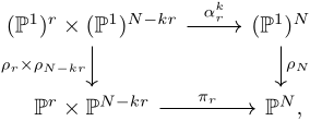
(A.1)

where α r k = ( Δ k ) × r × id ( P 1 ) N k r . We can use this diagram to have a concrete description of π r , ( h 0 h m ) . In order to do so, we first need the following lemma to describe the fundamental class of the image of α r k .

Lemma A.4

We have the identity

[ Δ k ] = j = 0 k 1 τ k 1 j σ j k ( h 1 , , h k )

in the Chow ring of ( P 1 ) × k for every k 2 , where σ j k ( ) is the elementary symmetric function with 𝑘 variables of degree 𝑗.

Proof

The diagonal Δ k is equal to the complete intersection of the hypersurfaces of ( P 1 ) k of equations x 0 , i x 1 , i + 1 x 0 , i + 1 x 1 , i for 1 i k 1 (we are denoting by x 0 , i , x i , 1 the two coordinates of the 𝑖-th factor of the product). Therefore, we have

Δ k = i = 1 k 1 ( h i + h i + 1 + τ ) .

Notice that, in the Chow ring of ( P 1 ) k , we have 𝑘 relations of degree 2 which can be written as h i 2 + τ h i = 0 for every i = 1 , , k .

The case k = 2 was already proven in [22, Lemma 3.8]. We proceed by induction on 𝑘. We have

Δ k + 1 = i = 1 k ( h i + h i + 1 + τ ) = ( h k + 1 + h k + τ ) Δ k ,

and thus, by induction,

Δ k + 1 = i = 0 k 1 h k + 1 τ k 1 i σ i k + i = 0 k 1 τ k i σ i k + i = 0 k 1 h k τ k 1 i σ i k .

Recall that we have the relations

σ j k ( x 1 , , x k ) = x k σ j 1 k 1 ( x 1 , , x k 1 ) + σ j k 1 ( x 1 , , x k 1 )

between elementary symmetric functions (with σ j k = 0 for j > k ); therefore, we have

i = 0 k 1 τ k 1 i h k σ i k = i = 0 k 1 τ k 1 i ( h k 2 σ i 1 k 1 + h k σ i k 1 ) = i = 0 k 1 τ k 1 i h k ( τ σ i 1 k 1 + σ i k 1 ) ,

where we used the relation h k 2 + τ h k = 0 in the last equalities. Therefore, we get

Δ k + 1 = i = 0 k 1 τ k 1 i ( h k + 1 σ i k + h k σ i k 1 ) + i = 0 k 1 τ k i ( σ i k h k σ i 1 k 1 ) = i = 0 k 1 τ k 1 i ( h k + 1 σ i k + h k σ i k 1 ) + i = 0 k 1 τ k i σ i k 1 .

Shifting the index of the last sum, it is easy to get the following identity:

Δ k + 1 = h k + 1 σ k 1 k + h k σ k 1 k 1 + τ k + i = 0 k 2 τ k 1 i ( h k + 1 σ i k + h k σ i k 1 + σ i + 1 k 1 ) ,

and the statement follows from shifting the last sum again and from using the relations between the symmetric functions (notice that h k σ k 1 k 1 = σ k k ). ∎

Remark A.5

Define by θ m , r the 𝑇-equivariant closed subvariety of ( P 1 ) r × ( P 1 ) N k r of the form

θ m , r : = m + 1 × ( P 1 ) r ( m + 1 ) × ( P 1 ) N k r

induced by the 𝑇-equivariant closed immersion P 1 . We have that

( ρ r × ρ N k r ) ( θ m . r ) = ( r ( m + 1 ) ) ! ( N k r ) ! h 0 h m

for every m r 1 .

From now on, we set d : = r ( m + 1 ) 0 . Thanks to the remark and the commutativity of diagram (A.1), we can compute the pushforward ρ N , α r , k ( θ m , r ) and then divide it by d ! ( N k r ) ! to get π r , ( h 0 h m ) .

We denote by α l ( k , d ) the integer

α l ( k , d ) : = j 1 + + j d = l 0 j s k 1 ( k j 1 ) ( k j d )

and by β l ( k , m , r ) the integer (because l d ( k 1 ) )

β l ( k , m , r ) : = ( N ( m + 1 ) k l ) ! ( N k r ) ! d ! .

Lemma A.6

We get the equality

π r , ( h 0 h m ) = l = 0 d ( k 1 ) α l ( k , d ) β l ( k , m , r ) τ d ( k 1 ) l h 0 h ( m + 1 ) k + l 1

in the 𝑇-equivariant Chow ring of P N .

Proof

Thanks to Lemma A.4, we have that

α r , k ( θ m , r ) = [ k ( m + 1 ) × ( Δ k ) d × ( P 1 ) N k r ] = h 1 h ( m + 1 ) k i = 1 d ( j = 0 k 1 τ k 1 j σ j k ( h ( m + j ) k + 1 , h ( m + j ) k + 2 , , h ( m + j + 1 ) k ) ) ;

we need to take the image through ρ N , of this element. However, we have that

ρ N , ( h i 1 h i s ) = ρ N , ( h 1 h s )

for every 𝑠-tuple ( i 1 , , i s ) of distinct indexes because ρ N is an S N -quotient. Therefore, a simple computation shows that ρ N , α r , k ( θ m , r ) has the following form:

l = 0 d ( k 1 ) ( j 1 + + j d = l 0 j s k 1 ( k j 1 ) ( k j d ) ) ( N ( m + 1 ) k l ) ! τ d ( k 1 ) l h 0 h ( m + 1 ) k + l 1 .

The statement follows. ∎

Remark A.7

Notice that the expression makes sense also per m = 1 , and in fact, we get a description of the π r , ( 1 ) .

Let us describe the case r = 1 . Clearly, we only have d = 1 (or m = 1 ) and d = 0 (or m = 0 ). If d = 0 , the formula gives us

π 1 , ( h 0 ) = h 0 h k 1 CH T ( P N ) ;

if d = 1 a simple computation shows

π 1 , ( 1 ) = l = 0 k 1 ( k l ) ! ( k l ) ( N k N l ) τ k 1 l h 0 h l 1 CH T ( P N ) .

These two formula give us the 𝑇-equivariant class of these two elements. As matter of fact, π 1 , ( 1 ) is also a GL 2 -equivariant class by definition. As far as π 1 , ( h 0 ) is concerned, this is clearly not GL 2 -equivariant. Nevertheless, we can consider π 1 , ( ξ 1 ) = π 1 , ( h 0 ) + t 1 π 1 , ( 1 ) , which is a GL 2 -equivariant class.

We can describe π 1 , ( 1 ) geometrically. In fact, it is the fundamental class of the locus describing forms 𝑓 such that 𝑓 has a root with multiplicity at least 𝑘. This locus is strictly related to locus of A k -singularities in the moduli stack of cyclic covers of the projective line of degree 2.

We denote by 𝐼 the ideal generated by the two elements described in the previous remark. First of all, we prove that almost all the pushforwards we need to compute are in this ideal.

Proposition A.8

We have that

π r , ( h 0 h m ) I

for every 1 r N / k and 0 m r 1 .

Proof

Lemma A.6 implies that it is enough to prove that ( m + 1 ) k + l 1 k 1 for every l = 0 , , d ( k 1 ) , where d = r ( m + 1 ) , because it implies that every factor of π r , ( h 0 h m ) is divisible by h 0 h k 1 . This follows from m 0 . ∎

Therefore, it only remains to prove that π r , ( 1 ) is in the ideal 𝐼 for r 2 . To do so, we need to prove some preliminary results.

Proposition A.9

We have the equality

h 0 2 h n 1 2 h n h m 1 = s = 0 n ( 1 ) s s ! ( n s ) ( m s ) τ s h 0 h m + n s 1

in the 𝑇-equivariant Chow ring of P N for every n m .

Proof

Denote by x n , m the left term of the equality. Because we have the identity h i = h j + ( j i ) τ in the 𝑇-equivariant Chow ring of P N , we have the following formula:

x n , m = x n 1 , m + 1 ( m n + 1 ) τ x n 1 , m ,

which gives us that x n , m is uniquely determined from the elements x 0 , j for j N . This implies that it is enough to prove that the formula in the statement verifies the recursive formula above. This follows from straightforward computation. ∎

Before going forward with our computation, we recall the following combinatorial fact.

Lemma A.10

For every pair of non-negative integers k , m N , we have that

l = 0 k 1 ( 1 ) l ( m l ) ( N l k 1 l ) = ( N m k 1 ) .

We are going to use it to prove the following result.

Proposition A.11

For every non-negative integer t k 1 , we have the equality

h 0 h t 1 π 1 , ( 1 ) = f = 0 k 1 ( N f t ) ! ( N k t ) ! ( k f ) τ k 1 f h 0 h t + f 1 + I

in the 𝑇-equivariant Chow ring of P N . Again, for t = 0 , we end up with the formula for π 1 , ( 1 ) .

Proof

The left-hand side of the equation in the statement can be written as

l = 0 t ( k l ) ! ( k l ) ( N k N l ) τ k 1 l h 0 2 h l 1 2 h l h t 1 + l = t + 1 k 1 ( k l ) ! ( k l ) ( N k N l ) τ k 1 l h 0 2 h t 1 2 h t h l 1 ;

see Remark A.7. If we apply Proposition A.9 to the two sums, we get

l = 0 t s = 0 l ( 1 ) s k ! ( N l ) ! t ! ( k l ) ! ( N k ) ! s ! ( l s ) ! ( t s ) ! τ k 1 l + s h 0 h l + t s 1 , l = t + 1 t s = 0 t ( 1 ) s k ! ( N l ) ! t ! ( k l ) ! ( N k ) ! s ! ( l s ) ! ( t s ) ! τ k 1 l + s h 0 h l + t s 1 ;

if we exchange the sums in each factor and put everything together, we end up with

s = 0 t l = s k 1 ( 1 ) s k ! ( N l ) ! t ! ( k l ) ! ( N k ) ! s ! ( l s ) ! ( t s ) ! τ k 1 l + s h 0 h l + t s 1 .

Shifting the inner sum and setting f : = l s , we get

s = 0 t f = 0 k 1 s ( 1 ) s k ! ( N s f ) ! t ! ( k s f ) ! ( N k ) ! s ! f ! ( t s ) ! τ k 1 f h 0 h l + f 1 .

Notice that we can extend the inner sum up to k 1 as all the elements we are adding are in the ideal 𝐼. Therefore, we exchange the sums again and get

f = 0 k 1 ( 1 ) s k ! f ! τ k 1 f h 0 h l + f 1 ( s = 0 t ( 1 ) s ( N s f k s f ) ( t s ) ) + I ,

and we can conclude using Lemma A.10. ∎

We state now the last technical lemma.

Lemma A.12

If we define Γ t to be the element

( N t ) ! ( N 2 k + 1 ) ! τ 2 ( k 1 ) t h 0 h t 1

in the 𝑇-equivariant Chow ring of P N , we have that Γ t I for every t k 1 .

Proof

We proceed by induction on m = k 1 t . The case m = 0 follows from the previous proposition.

Suppose that Γ s I for every s k t . If we consider the element in 𝐼,

( N k t ) ! ( N 2 k + 1 ) ! τ k 1 t h 0 h t 1 π 1 , ( 1 ) ,

we can apply the previous proposition again and get

f = 0 k 1 ( k f ) ( N f t ) ! ( N 2 k + 1 ) ! τ 2 ( k 1 ) ( f + t ) h 0 h t + f 1 I ,

which is the same as

f = 0 k 1 ( k f ) Γ f + t I .

The statement follows by induction. ∎

Remark A.13

It is important to notice that more is true; the same exact proof shows us that

Γ t ( 2 ( k 1 ) t k 1 t ) I

for every t k 1 . This will not be needed, except for the case t = 0 , where this implies that in particular Γ 0 2 I .

Before going to prove the final proposition, we recall the following combinatorial fact.

Lemma A.14

We have the numerical equality

j 1 + + j r = l 0 j s k 1 ( k j 1 ) ( k j r ) = ( r k l )

for every l k 1 . In particular, in our situation, we have

α l ( k , r ) = ( r k l )

for l k 1 .

Finally, we are ready to prove the last statement.

Proposition A.15

We have π r , ( 1 ) is contained in the ideal 𝐼 for r 2 .

Proof

Notice that

π r , ( 1 ) = l = 0 r ( k 1 ) α l ( k , r ) β l ( k , 1 , r ) τ r ( k 1 ) l h 0 h l 1 = l = 0 k 1 α l ( k , r ) β l ( k , 1 , r ) τ r ( k 1 ) l h 0 h l 1 + I ;

therefore, we have to study the first k 1 elements of the sum. Using Lemma A.14, we get the following chain of equalities modulo the ideal I:

π r , ( 1 ) = l = 0 k 1 ( r k l ) ( N l ) ! ( N r k ) ! r ! τ r ( k 1 ) l h 0 h l = l = 0 k 1 ( r k l ) ( N 2 k + 1 ) ! ( N r k ) ! r ! τ ( r 2 ) ( k 1 ) Γ l ;

therefore, it remains to prove that the coefficient

( r k l ) ( N 2 k + 1 ) ! ( N r k ) ! r !

is an integer for every r 2 and any l k 1 . First of all, we notice that this is the same as

( r k l ) ( N r k + r r ) ( N 2 k + 1 ) ! ( N r k + r ) ! ,

which implies that, for r 3 and l k 1 , this is an integer. It remains to prove the statement for r = 2 , i.e. to prove that the number

( 2 k l ) N 2 k + 1 2

is an integer. Notice that it is clearly true for l 1 but not for l = 0 . However, we have that Γ 0 2 I by Remark A.13; therefore, we are done. ∎

Corollary A.16

The image of CH ( Δ k ) CH ( P N ) is the ideal generated by the two elements π 1 , ( 1 ) and π 1 , ( h 0 ) . See Remark A.7 for the explicit description.

References

[1] D. Abramovich, M. Olsson and A. Vistoli, Twisted stable maps to tame Artin stacks, J. Algebraic Geom. 20 (2011), no. 3, 399–477. 10.1090/S1056-3911-2010-00569-3Search in Google Scholar

[2] A. Arsie and A. Vistoli, Stacks of cyclic covers of projective spaces, Compos. Math. 140 (2004), no. 3, 647–666. 10.1112/S0010437X03000253Search in Google Scholar

[3] S. Canning and H. Larson, The Chow rings of the moduli spaces of curvesof genus 7, 8, and 9, J. Algebraic Geom. 33 (2024), 55–116. 10.1090/jag/818Search in Google Scholar

[4] A. Di Lorenzo, D. Fulghesu and A. Vistoli, The integral Chow ring of the stack of smooth non-hyperelliptic curves of genus three, Trans. Amer. Math. Soc. 374 (2021), no. 8, 5583–5622. 10.1090/tran/8354Search in Google Scholar

[5] A. Di Lorenzo, M. Pernice and A. Vistoli, Stable cuspidal curves and the integral Chow ring of M ̄ 2 , 1 , preprint (2021), https://arxiv.org/abs/2108.03680. Search in Google Scholar

[6] A. Di Lorenzo and A. Vistoli, Polarized twisted conics and moduli of stable curves of genus two, preprint (2021), https://arxiv.org/abs/2103.13204. Search in Google Scholar

[7] D. Edidin and D. Fulghesu, The integral Chow ring of the stack of at most 1-nodal rational curves, Comm. Algebra 36 (2008), no. 2, 581–594. 10.1080/00927870701719045Search in Google Scholar

[8] D. Edidin and D. Fulghesu, The integral Chow ring of the stack of hyperelliptic curves of even genus, Math. Res. Lett. 16 (2009), no. 1, 27–40. 10.4310/MRL.2009.v16.n1.a4Search in Google Scholar

[9] D. Edidin and W. Graham, Equivariant intersection theory, Invent. Math. 131 (1998), no. 3, 595–634. 10.1007/s002220050214Search in Google Scholar

[10] J. Elliott, Factoring formal power series over principal ideal domains, Trans. Amer. Math. Soc. 366 (2014), no. 8, 3997–4019. 10.1090/S0002-9947-2014-05903-5Search in Google Scholar

[11] E. Esteves, The stable hyperelliptic locus in genus 3: An application of Porteous formula, J. Pure Appl. Algebra 220 (2016), no. 2, 845–856. 10.1016/j.jpaa.2015.07.020Search in Google Scholar

[12] C. Faber, Chow rings of moduli spaces of curves. I. The Chow ring of M ̄ 3 , Ann. of Math. (2) 132 (1990), no. 2, 331–419. 10.2307/1971525Search in Google Scholar

[13] G. Inchiostro, Moduli of genus one curves with two marked points as a weighted blow-up, Math. Z. 302 (2022), no. 3, 1905–1925. 10.1007/s00209-022-03121-5Search in Google Scholar

[14] E. Izadi, The Chow ring of the moduli space of curves of genus 5, The moduli space of curves, Progr. Math. 129, Birkhäuser, Boston (1995), 267–304. 10.1007/978-1-4612-4264-2_10Search in Google Scholar

[15] E. Larson, The integral Chow ring of M ̄ 2 , Algebr. Geom. 8 (2021), no. 3, 286–318. 10.14231/AG-2021-007Search in Google Scholar

[16] D. Mumford, Towards an enumerative geometry of the moduli space of curves, Arithmetic and geometry, Vol. II, Progr. Math. 36, Birkhäuser, Boston (1983), 271–328. 10.1007/978-1-4757-9286-7_12Search in Google Scholar

[17] N. Penev and R. Vakil, The Chow ring of the moduli space of curves of genus six, Algebr. Geom. 2 (2015), no. 1, 123–136. 10.14231/AG-2015-006Search in Google Scholar

[18] M. Pernice, Hyperelliptic a r -stable curves (and their moduli stack), preprint (2023), https://arxiv.org/abs/2302.11456. 10.1090/tran/9164Search in Google Scholar

[19] M. Pernice, The (almost) integral chow ring of m ̃ 3 7 , preprint (2023), https://arxiv.org/abs/2303.05493. Search in Google Scholar

[20] M. Pernice, The moduli stack of a r -stable curves, preprint (2023), https://arxiv.org/abs/2302.10877. Search in Google Scholar

[21] M. Romagny, Group actions on stacks and applications, Michigan Math. J. 53 (2005), no. 1, 209–236. 10.1307/mmj/1114021093Search in Google Scholar

[22] A. Vistoli, The Chow ring of M 2 . Appendix to “Equivariant intersection theory”, Invent. Math. 131 (1998), no. 3, 635–644. 10.1007/s002220050215Search in Google Scholar

Received: 2023-06-21
Revised: 2024-04-15
Published Online: 2024-06-04
Published in Print: 2024-07-01

© 2024 the author(s), published by De Gruyter

This work is licensed under the Creative Commons Attribution 4.0 International License.

Downloaded on 15.9.2025 from https://www.degruyterbrill.com/document/doi/10.1515/crelle-2024-0034/html
Scroll to top button