Towards the cosymplectic topology

Stéphane Tchuiaga

doi:10.1515/coma-2022-0151

Article Open Access

Towards the cosymplectic topology

Stéphane Tchuiaga

Published/Copyright: July 18, 2023

Published by

Become an author with De Gruyter Brill

Submit Manuscript Author Information Explore this Subject

From the journal Complex Manifolds Volume 10 Issue 1

Abstract

In this article, the cosymplectic analogue of the symplectic flux homomorphism of a compact connected cosymplectic manifold ( M , η , ω ) with ∂ M = ∅ is studied. This is a continuous map with respect to the C 0 -metric, whose kernel is connected by smooth arcs and coincides with the subgroup of all weakly Hamiltonian diffeomorphisms. We discuss the cosymplectic analogue of the Weinstein’s chart, and derive that the group G η , ω ( M ) of all cosymplectic diffeomorphisms isotopic to the identity map is locally contractible. A study of an analogue of Polterovich’s regularization process for co-Hamiltonian isotopies follows. Finally, we study Moser’s stability theorems for locally conformal cosymplectic manifolds.

Keywords: Locally conformal cosymplectic manifolds; flux homomorphism; the Weinstein chart; diffeomorphisms; differential forms

MSC 2010: 53C24; 53C15; 53D05; 57R17

1 Introduction

Based on the work of Lichnerowicz [12] and the thesis of Gallissot [6] on exterior forms in mechanics, Libermann [11] gives for the first time a classification of differentiable varieties in odd dimension M 2 n + 1 . This classification gives rise to almost cosymplectic structures on this manifold, i.e., a differentiable manifold of odd dimension M 2 n + 1 admitting a 1-form η and a 2-form ω such that η ∧ ω n ≠ 0 , at each point of M 2 n + 1 : the pair ( η , ω ) is then called an almost cosymplectic structure of M 2 n + 1 . If for a given almost cosymplectic manifold ( M , η , ω ) , the 1-form η and the 2-form ω are both closed, then M is called a cosymplectic manifold. We emphasize that cosymplectic structures are special cases of stable Hamiltonian structures. Another work in this direction was introduced by Chinea et al. linking cosymplectic manifolds and time-dependent Hamiltonian systems [5]. Advanced studies of the structure of the group of cosymplectic diffeomorphisms and cosymplectic vector fields were carried out in previous studies [4,15,17].

The goal of this article is to continue the study of the identity component in the group of all cosymplectic diffeomorphisms of a closed cosymplectic manifold ( M , η , ω ) in parallel with some well established results found in symplectic geometry [1,3].

In the context of symplectic geometry, the corresponding isomorphism between vector fields and 1-forms induced by the symplectic structure is used to construct a surjective homomorphism called the flux homomorphism, which is deeply rooted in the description of some structures of the group of Hamiltonian diffeomorphisms of a closed symplectic manifold [1].

Yet, to the best of author’s knowledge, there is no well-known definition of the cosymplectic analogue of the symplectic flux homomorphism (e.g. we don’t know the cosymplectic analogue of the flux group).

In this article, we will attempt to define the concept of flux geometry on a closed cosymplectic manifold with the aid of symplectic topology.

The existence of such a homomorphism can be motivated as follows: From [17], it follows that the identity component (with respect to the compact-open topology [8]) in the group of all cosymplectic diffeomorphisms of a closed cosymplectic manifold ( M , η , ω ) is denoted G η , ω ( M ) . This subgroup contains a normal subgroup Ham η , ω ( M ) called the group of weakly Hamiltonian diffeomorphisms. Our wish is to realize the subgroup Ham η , ω ( M ) as the kernel of a group homomorphism (this is supported by a classical result from group theory). We organize this article as follows.

In Section 2, we recall the definitions of cosymplectic manifolds, cosymplectic vector spaces, and some comparison results are stated: Proposition 2.10, Lemma 2.11, and Lemma 2.13.

Section 3 deals with the construction and the study of the cosymplectic flux homomorphism. This section starts with the study of the cosymplectic analogue of the Weinstein chart: Lemma 3.2 constructs a surjective map from the first fundamental group π 1 ( G η , ω ( M ) ) of G η , ω ( M ) onto the first fundamental group π 1 ( M ) of a compact connected cosymplectic manifold ( M , η , ω ) , Lemma 3.3 shows that the group G η , ω ( M ) is locally contractible, and Proposition 3.4 exhibits the cosymplectic analogue of the Weinstein chart. In Section 3.2, we construct the cosymplectic flux homomorphism S ˜ η , ω : the surjective homomorphism S ˜ η , ω is invariant on a homotopy class (relatively to fixed endpoints) of each cosymplectic isotopy and is continuous with respect to the C 0 -compact open topology (Theorem 3.8) and Proposition 3.9 shows how the co-Weinstein chart is related to the cosymplectic flux homomorphism.

Section 4 deals with the study of a surjective group homomorphism S η , ω defined on G η , ω ( M ) : Proposition 4.1 states that ker S η , ω is connected by smooth arcs, Proposition 4.2 states that ker S η , ω coincides with the subgroup Ham η , ω ( M ) of all weakly Hamiltonian diffeomorphisms, Proposition 4.3 implies that the corresponding flux group Γ η , ω is countable, Proposition 4.4 links Γ η , ω to ker S η , ω , vice versa, and Lemma 4.5 states that any smooth cosymplectic isotopy in ker S η , ω is a weakly Hamiltonian isotopy. Also, Proposition 4.6 is a summary of the study of the co-flux homomorphism into a diagram of exact sequences.

In Section 5, we show that any co-Hamiltonian isotopy ψ F can be regularized to obtain another co-Hamiltonian isotopy ψ H such that both paths ψ F and ψ H have the same extremities. It follows that the restrictions of the two norms ‖ . ‖ Co ( 1 , ∞ ) and ‖ . ‖ Co ∞ defined in [17] coincide on Ham η , ω 0 ( M ) . Finally, in Section 6, we make use of the definition of locally conformal cosymplectic manifolds introduced in [5] to study cosymplectic stability. The main result of this section is Theorem 6.2.

2 Preliminaries

2.1 Cosymplectic vector spaces

Let V be a vector space. Given any non-trivial linear map ψ : V ⟶ R , together with a bilinear map b : V × V ⟶ R , one defines a linear map:

I ˜ ψ , b : V ⟶ V ∗ v ⟼ I ˜ ψ , b ( v ) ≔ i v b + ψ ( v ) ψ

so that I ˜ ψ , b ( v ) ( u ) = b ( v , u ) + ψ ( v ) ψ ( u ) , for all u , v ∈ V .

Definition 2.1

[17]

A pair ( b , ψ ) consisting of an antisymmetric bilinear map b : V × V ⟶ R and a non-trivial linear map ψ : V ⟶ R is called cosymplectic structure if the map I ˜ ψ , b is a bijection such that the Reeb vector ξ ≔ I ˜ ψ , b − 1 ( ψ ) satisfies b ( ξ , v ) = 0 for all v ∈ V .
A cosymplectic vector space is a triple ( V , b , ψ ) , where V is a vector space and ( b , ψ ) is a cosymplectic structure on V .

2.2 Cosymplectic manifolds

Let M be a smooth manifold of dimension 2 n + 1 . An almost cosymplectic structure on M is a pair ( ω , η ) consisting of a 2-form ω and a 1-form η such that for each x ∈ M , the triple ( T x M , ω x , η x ) is a cosymplectic vector space. Therefore, a cosymplectic structure on M is any almost cosymplectic structure ( ω , η ) on M such that d η = 0 and d ω = 0 . We shall write ( M , ω , η ) to mean that M has a cosymplectic structure ( ω , η ) . For further details, we refer to [7,11,17] and references therein. Any cosymplectic manifold ( M , η , ω ) is orientable with respect to the volume form η ∧ ω n , any cosymplectic manifold ( M , η , ω ) admits a vector field ξ called the Reeb vector field such that η ( ξ ) = 1 , and ι ξ ω = 0 [17]. Also, not all odd dimensional manifolds have a cosymplectic structure ([17], Li [7]). We refer the reader to [17] for further details.

2.3 Vector fields and cosymplectic structure [17]

Definition 2.2

Let ( M , η , ω ) be a cosymplectic manifold. A vector field X is said to be cosymplectic if ℒ X η = 0 and ℒ X ω = 0 .

We shall denote by χ η , ω ( M ) the space of all cosymplectic vector fields of ( M , ω , η ) .

Definition 2.3

Let ( M , η , ω ) be a cosymplectic manifold. An element Y ∈ χ η , ω ( M ) is called a weakly Hamiltonian vector field if the 1-form I ˜ η , ω ( Y ) is exact.

We shall denote by ham η , ω ( M ) the space of all weakly Hamiltonian vector fields of ( M , η , ω ) .

Definition 2.4

Let ( M , η , ω ) be a cosymplectic manifold. An element Y ∈ χ η , ω ( M ) is called a co-Hamiltonian vector field if the 1-form ι Y ω is exact, and η ( Y ) = 0 .

We shall denote by ham η , ω 0 ( M ) the space of all co-Hamiltonian vector fields of ( M , η , ω ) .

Definition 2.5

Let ( M , η , ω ) be a cosymplectic manifold. A diffeomorphism ϕ : M ⟶ M is called a cosymplectic diffeomorphism (or cosymplectomorphism) if ϕ ∗ ( η ) = η and ϕ ∗ ( ω ) = ω .

We shall denote by Cosymp η , ω ( M ) the space of all cosymplectomorphisms of ( M , ω , η ) .

Definition 2.6

Let ( M , η , ω ) be a cosymplectic manifold. An isotopy Φ = { ϕ t } is called a cosymplectic isotopy if for each time t , we have ϕ t ∈ Cosymp η , ω ( M ) .

We shall denote by Iso η , ω ( M ) the space of all almost cosymplectic isotopies of ( M , η , ω ) . We shall need the following important subgroup:

G η , ω ( M ) ≔ ev 1 ( Iso η , ω ( M ) ) ,

and equip G η , ω ( M ) with the C ∞ -compact-open topology [8].

Definition 2.7

Let ( M , η , ω ) be a cosymplectic manifold. An isotopy Ψ ≔ { ψ t } is called a weakly Hamiltonian isotopy, if for each t , the vector field ψ ˙ t is a weakly Hamiltonian vector field, i.e., ψ ˙ t ∈ ham η , ω ( M ) .

We shall denote by H η , ω ( M ) the space of all weakly Hamiltonian isotopies of ( M , ω , η ) and put

(2.1) Ham η , ω ( M ) ≔ ev 1 ( H η , ω ( M ) ) .

The elements of the set Ham η , ω ( M ) are called weakly Hamiltonian diffeomorphisms of ( M , ω , η ) .

Definition 2.8

Let ( M , η , ω ) be a cosymplectic manifold. An isotopy Ψ ≔ { ψ t } is called a co-Hamiltonian isotopy, if for each t , the vector field ψ ˙ t is a co-Hamiltonian vector field, i.e., ψ ˙ t ∈ ham η , ω 0 ( M ) .

We shall denote by H η , ω 0 ( M ) the space of all co-Hamiltonian isotopies of ( M , η , ω ) and put

(2.2) Ham η , ω 0 ( M ) ≔ ev 1 ( H η , ω 0 ( M ) ) .

It is clear that we have the inclusion Ham η , ω 0 ( M ) ⊆ Ham η , ω ( M ) . Furthermore, if we have a compact connected cosymplectic manifold, then Ham η , ω 0 ( M ) = Ham η , ω ( M ) , provided the flow generated by the Reed vector field has at least a closed orbit.

2.4 Formula for composition of cosymplectic paths [17]

We have the following properties.

Let { ϕ t } ∈ H η , ω 0 ( M ) such that I ˜ η , ω ( ϕ ˙ t ) = d F t , for each t and smooth function F t . Then, we have
(2.3) I ˜ η , ω ( ϕ t − 1 ︷ ˙ ) = − ϕ t ∗ ( ι ϕ ˙ t ω ) − ϕ t ∗ ( η ( ϕ ˙ t ) ) η = − ϕ t ∗ ( I ˜ η , ω ( ϕ ˙ t ) ) = d ( − F t ∘ ϕ t ) ,
for all t , where ϕ t − 1 is the inverse map of ϕ t . To simplify the notations in computation, w.l.o.g we might denote the inverse map of ϕ t as ϕ − t .
If Φ F = { ϕ t } is a co-Hamiltonian isotopy such that I ˜ η , ω ( ϕ ˙ t ) = d F t , for all t , then for all ρ ∈ G η , ω ( M ) , the isotopy Ψ = { ψ t } with ψ t ≔ ρ − 1 ∘ ϕ t ∘ ρ is also co-Hamiltonian: in fact, from ψ ˙ t = ρ ∗ − 1 ( ϕ ˙ t ) , we derive that
(2.4) I ˜ η , ω ( ψ ˙ t ) = ρ ∗ ( I ˜ η , ω ( ϕ ˙ t ) ) = d ( F t ∘ ρ ) , for each t .
Similarly, if { ψ t } and { ϕ t } are two elements of H η , ω 0 ( M ) such that I ˜ η , ω ( ϕ ˙ t ) = d F t and I ˜ η , ω ( ψ ˙ t ) = d K t , for each t , then we have
(2.5) I ˜ η , ω ( ϕ t ∘ ψ t ︷ ˙ ) = d ( F t + K t ∘ ϕ t − 1 ) , for each t .
Let { ϕ t } ∈ Iso η , ω ( M ) . Then, for each t , we have
(2.6) I ˜ η , ω ( ϕ ˙ − t ) = − ϕ t ∗ ( I ˜ η , ω ( ϕ ˙ t ) ) .
If { ψ t } and { ϕ t } are two elements of Iso η , ω ( M ) , then for each t , we have
(2.7) I ˜ η , ω ( ϕ t ∘ ψ t ︷ ˙ ) = I ˜ η , ω ( ϕ ˙ t ) + ( ϕ t − 1 ) ∗ ( I ˜ η , ω ( ψ ˙ t ) ) .

We shall often use the following important result in this article without mentioning it.

Lemma 2.9

[7,10] Let M be a manifold and η and ω be two differential forms on M with degrees 1 and 2, respectively. Consider M ˜ = M × R equipped with the 2-form ω ˜ ≔ p ∗ ( ω ) + p ∗ ( η ) ∧ π 2 ∗ ( d u ) , where u is the coordinate function on R , p : M ˜ ⟶ M , and π 2 : M ˜ ⟶ R , are canonical projections. Then, ( M , η , ω ) is a cosymplectic manifold if and only if ( M ˜ , ω ˜ ) is a symplectic manifold.

2.5 The C 0 -topology

Let Homeo ( M ) denote the group of all homeomorphisms of M equipped with the C 0 -compact-open topology. This is the metric topology induced by the distance d 0 M ( f , h ) = max ( d C 0 ( f , h ) , d C 0 ( f − 1 , h − 1 ) ) , where d C 0 ( f , h ) = sup x ∈ M d ( h ( x ) , f ( x ) ) . On the space of all continuous paths λ : [ 0 , 1 ] → Homeo ( M ) such that λ ( 0 ) = id M , we consider the C 0 -topology as the metric topology induced by the metric d ¯ M ( λ , μ ) = max t ∈ [ 0 , 1 ] d 0 M ( λ ( t ) , μ ( t ) ) .

2.6 Comparison of some norms

Consider a 1- form α on M and let us recall the definition of the supremum norm (i.e., the uniform sup norm) of α : for each x ∈ M , we know that α induces a linear map α x : T x M → R , whose norm is given by:

(2.8) ‖ α x ‖ g M ≔ sup { ∣ α x ( X ) ∣ ; X ∈ T x M , ‖ X ‖ g M = 1 } ,

where ‖ ⋅ ‖ g M is the norm induced on each tangent space T x M (at the point x ) by the Riemannian metric g M . Therefore, the uniform sup norm of α , say ∣ ⋅ ∣ 0 , is defined as:

(2.9) ∣ α ∣ 0 ≔ sup x ∈ M ‖ α x ‖ g M .

Proposition 2.10

Let M and N be two smooth compact connected Riemannian manifolds. We have

∣ p ∗ ( α ) ∣ 0 = ∣ α ∣ 0 ,

i.e., the projection map p : M × N → M , induces a map p ∗ , which preserves the C 0 -norm.

2.6.1 The Hodge norm

Given a Riemannian metric g on an oriented manifold M , let d V ol g denote the volume element induced by the Riemannian metric, and by ♭ the isomorphism induced by the metric g from the space of vector fields and that of all 1-forms so that ♭ ( X ) ≔ ι X g . The inverse mapping of ♭ will be denoted ♯ . So, one can equip the space of 1-forms with a metric tensor g ˜ defined by g ˜ ( α 1 , α 2 ) ≔ g ( ♯ α 1 , ♯ α 2 ) , for all differential 1-forms α 1 , and α 2 . Thus, the L 2 -Hodge norm of α is defined by:

(2.10) ‖ α ‖ L 2 2 ≔ ∫ M g ( ♯ α , ♯ α ) d V ol g .

Let H 1 ( M , R ) (resp. H 1 ( M ˜ , R ) ) denote the first de Rham cohomology group (with real coefficients) of M (resp. M ˜ ), and let Z 1 ( M ) (resp. Z 1 ( M ˜ ) ) denote the space of all closed 1-forms on M (resp. M ˜ ) [14,18]. The L 2 -Hodge norm of a de Rham cohomology class [ α ] of a closed 1-form α is then defined as the norm ‖ ℋ α ‖ L 2 , where ℋ α is the harmonic representative of [ α ] . Consider the map

(2.11) S : H 1 ( M , R ) ⟶ Z 1 ( M )

to be a fixed linear section of the natural projection π M : Z 1 ( M ) ⟶ H 1 ( M , R ) . Each α ∈ Z 1 ( M ) splits as:

(2.12) α = S ( π M ( α ) ) + ( α − S ( π M ( α ) ) ) .

We shall call the 1-form ( α − S ( π M ( α ) ) ) the exact part of α and throughout this article, for simplicity, when this will be necessary, the latter 1-form will be denoted d f α , S to mean that it is the differential of a certain function that depends on α and S ; however, we shall call the 1-form S ( π M ( α ) ) the S -form of α . Let H 1 ( M , S ) denote the space of all S -forms and define the set B 1 ( M ) as : B 1 ( M ) ≔ ( Z 1 ( M ) \ H 1 ( M , S ) ) ∪ { 0 } . We then have the following direct sum : Z 1 ( M ) = H 1 ( M , S ) ⊕ S B 1 ( M ) , with dim ( H 1 ( M , S ) ) = dim ( H 1 ( M , R ) ) < ∞ , for each linear section S (see [14,16,18]). Denote by P H 1 ( M , S ) the space of all smooth mappings ℋ : [ 0 , 1 ] → H 1 ( M , S ) . Since the spaces H 1 ( M , S ) and H 1 ( M , R ) are isomorphic and H 1 ( M , R ) is a finite dimensional vector space whose dimension is the first Betti number b 1 ( M ) , then H 1 ( M , S ) is of finite dimension [14]. Thus, there exist positive constants k 1 ( g ) and k 2 ( g ) , which depend on the Riemannian metric g on M such that

(2.13) k 1 ( g ) ‖ α ‖ L 2 ⩽ ∣ α ∣ 0 ⩽ k 2 ( g ) ‖ α ‖ L 2

for all α ∈ H 1 ( M , S ) . On the other hand, consider the projection p : M ˜ ⟶ M , and let

(2.14) π M ˜ : Z 1 ( M ˜ ) ⟶ H 1 ( M ˜ , R )

be the canonical projection, where Z 1 ( M ˜ ) is the set of all closed 1-forms on M ˜ : we have a commutative diagram

Z 1 ( M ) ⟶ p ∗ Z 1 ( M ˜ ) π M ↓ ↓ π M ˜ H 1 ( M , R ) ⟶ p ∗ H 1 ( M ˜ , R ) ,

namely p ∗ ∘ π M = π M ˜ ∘ p ∗ . Also, for any [ α ] ∈ H 1 ( M , R ) , we will often consider its following norm:

(2.15) ∣ [ α ] ∣ 0 ′ ≔ ∣ S ( π M ( α ) ) ∣ 0 .

Any norm on H 1 ( M , R ) is equivalent to the norm ∣ ⋅ ∣ 0 ′ .

We have the following facts.

Lemma 2.11

Let M and N be two smooth manifolds and q : M × N ⟶ M be the first projection, and y 0 ∈ N fixed. Then, for all vector field X on M × N , and for any l -form α on M, we have

(2.16) ι ( q ∗ X ) α = S y 0 ∗ ( ι ( X ) q ∗ ( α ) ) ,

where q ∗ X is the vector field on M defined by: For all f ∈ C ∞ ( M ) , q ∗ X ( f ) ≔ X ( f ∘ p ) ∘ S y 0 , and S y 0 : M → M × N , x ↦ ( x , y 0 ) (a section of q).

Proof

Consider a vector field X on M × N and y 0 ∈ N fixed. Let α be any l -form on M . For vector fields X 1 , … , X l − 1 on M , then ( S y 0 ) ∗ X i are vector fields, on M × N , and we have

(2.17) ι ( X ) q ∗ ( α ) ( ( S y 0 ) ∗ X 1 , … , ( S y 0 ) ∗ X l − 1 ) = q ∗ ( α ) ( X , ( S y 0 ) ∗ X 1 , … , ( S y 0 ) ∗ X l − 1 ) = α ( q ∗ X , X 1 , … , X l − 1 ) ∘ q = ι ( q ∗ X ) α ( X 1 , … , X l − 1 ) ,

modulo y 0 .□

Lemma 2.12

Let M and N be two smooth compact manifolds such that M × N has a volume form ω M × N , and q : M × N ⟶ M be the first projection. Let α be any S -form on M , and K be the S ˜ -part of q ∗ ( α ) , where S ˜ is any linear section of the natural projection

(2.18) π M × N : Z 1 ( M × N ) ⟶ H 1 ( M × N , R ) .

Let δ ( q , α ) be a function of mean zero such that d δ ( q , α ) = q ∗ ( α ) − K . Then, the map

(2.19) H 1 ( M , S ) ⟶ C ∞ ( M × N ) , α ↦ δ ( q , α )

is linear, and there exists a universal constant ϒ such that sup x ∈ M × N ∣ δ ( q , α ) ( x ) ∣ ≤ ϒ ‖ α ‖ L 2 .

Proof

Linearity: Compute

(2.20) d δ ( q , α + β ) = q ∗ ( α + β ) − S ˜ ( π M × N ( q ∗ ( α ) + q ∗ ( β ) ) ) = q ∗ ( α ) − S ˜ ( π M × N ( q ∗ ( α ) ) ) + q ∗ ( β ) − S ˜ ( π M × N ( q ∗ ( β ) ) ) = d δ ( q , β ) + d δ ( q , α ) .

That is, δ ( q , α + β ) = δ ( q , β ) + δ ( q , α ) + c t e . Since these functions have mean zero, then integrating this equality over M × N implies c t e = 0 . Hence, δ ( q , α + β ) = δ ( q , β ) + δ ( q , α ) . Continuity: Since H 1 ( M , S ) is a finite dimensional vector space, then any linear map from H 1 ( M , S ) to any other vector space is continuous: there exists a universal constant ϒ such that sup x ∈ M × N ∣ δ ( q , α ) ( x ) ∣ ≤ ϒ ‖ α ‖ L 2 .□

Lemma 2.13

Let M be a smooth compact manifold equipped with a Riemannian metric g, and q : M × S 1 ⟶ M be the first projection. Then,

the map q ∗ : Z 1 ( M ) → Z 1 ( M × S 1 ) , α ↦ q ∗ ( α ) , preserves the L 2 -Hodge norm up to multiplicative 2 π with respect to the product metric on M × S 1 .
if we equip H 1 ( M , R ) (resp. H 1 ( M × S 1 , R ) ) with any norm ∣ ⋅ ∣ (resp. ∣ . ∣ ’), then there exists a positive constant δ 0 (which depends on the norms ∣ ⋅ ∣ and ∣ . ∣ ’) such that ∣ [ α ] ∣ ≤ δ 0 ∣ [ q ∗ α ] ∣ ′ .

Proof

Let π 2 : M × S 1 ⟶ S 1 be the second projection onto S 1 , and h be the Riemannian metric on S 1 . The product metric on M × S 1 is defined as g ˜ ≔ q ∗ ( g ) + π 2 ∗ ( h ) . Let α ∈ Z 1 ( M ) , and set X α ≔ ♯ α and Y q ≔ ♯ q ∗ α . Consider the smooth section S 1 of the projection q such that S 1 ( x ) = ( x , 1 ) for all x ∈ M , where 1 ∈ S 1 , and compute

(2.21) q ∗ ( α ) = ι Y q g ˜ = ι Y q q ∗ ( g ) + ι Y q ( π 2 ) ∗ ( h ) = q ∗ ( ι q ∗ Y q g ) + π 2 ∗ ( ι ( π 2 ) ∗ Y q h ) .

Composing the aforementioned equality with S 1 ∗ gives: α = ι q ∗ Y q g , i.e., X α = q ∗ Y q mod 1 . Thus,

(2.22) ∫ M × S 1 g ˜ ( Y q , Y q ) d V ol g ˜ = ∫ M × S 1 α ( q ∗ Y q ) ∘ q d V ol g ˜ = ∫ M × S 1 α ( X α ) ∘ q d V ol g ˜ = ∫ M × S 1 g ( X α , X α ) ∘ q d V ol g ˜ = ∫ M × S 1 g ˜ ( Y q , Y q ) d V ol g ˜ = 2 π ∫ M g ( X α , X α ) d V ol g .

This implies that, ‖ q ∗ α ‖ L 2 = 2 π ‖ α ‖ L 2 . On the other hand, consider the linear map

L 0 : H 1 ( M × S 1 , R ) → H 1 ( M , R ) , [ β ] ↦ [ S 1 ∗ ( β ) ] ,

and derive from the continuity of L 0 that there exists a positive constant δ 0 such that ∣ L 0 ( [ β ] ) ∣ ≤ δ 0 ∣ [ β ] ∣ ′ . In particular, since p ∗ ( α ) ∈ Z 1 ( M × S 1 ) , for all α ∈ Z 1 ( M ) , we derive that ∣ L 0 ( [ q ∗ α ] ) ∣ ≤ δ 0 ∣ [ q ∗ α ] ∣ ′ , but L 0 ( [ q ∗ α ] ) = [ S 1 ∗ ( q ∗ α ) ] = [ ( q ∘ S 1 ) ∗ ( α ) ] = [ α ] : one obtains ∣ [ α ] ∣ ≤ δ 0 ∣ [ q ∗ α ] ∣ ′ .□

3 The co-flux geometry

3.1 Some structures of G η , ω ( M )

The studies concerned with this subsection will need the following result found in [17].

Proposition 3.1

[17]. Let ( M , η , ω ) be a compact cosymplectic manifold. If Φ F = { ϕ t } is any weakly Hamiltonian (resp. cosymplectic) isotopy such that I ˜ η , ω ( ϕ ˙ t ) = d F t , for all t, then the isotopy Φ ˜ = { ϕ ˜ t } defined by:

(3.1) ϕ ˜ t : M × S 1 ⟶ M × S 1 , ( x , θ ) ↦ ( ϕ t ( x ) , ℛ Λ t ( Φ F ) ( x , θ ) ) ,

is a Hamiltonian (resp. symplectic) isotopy of the symplectic manifold ( M ˜ , Ω ) with Hamiltonian F ˜ t ≔ F t ∘ p + p ∗ ( ι ( ϕ ˙ t ) η ) π 2 , where

(3.2) ℛ Λ t ( Φ ) ( x , θ ) ≔ θ − ∫ 0 t η ( ϕ ˙ s ) ∘ ϕ s ( x ) d s mod 2 π ,

with M ˜ ≔ M × S 1 , p : M ˜ → M , and π 2 : M ˜ → S 1 , are projection maps. Conversely, if the map

(3.3) ϕ ˜ t : M × S 1 ⟶ M × S 1 , ( x , θ ) ↦ ( ϕ t ( x ) , ℛ Λ t ( Φ F ) ( x , θ ) )

is a Hamiltonian (resp. symplectic) isotopy of the symplectic manifold ( M ˜ , Ω ) with Hamiltonian F ˜ , then the path t ↦ ϕ t is a weakly Hamiltonian (resp. cosymplectic) isotopy of ( M , η , ω ) with weak Hamiltonian H ˜ t ∘ S l , where S l : x ↦ ( x , l ) is any section of the projection π 2 .

We have the following results.

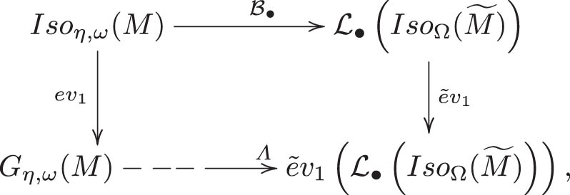
Lemma 3.2

Let ( M , η , ω ) be a connected compact cosymplectic manifold equipped with a Riemannian metric g. Then, there exists a surjective homomorphism co -ev from π 1 ( G η , ω ( M ) ) onto π 1 ( M ) .

Proof

Consider the compact symplectic manifold M ˜ ≔ M × S 1 equipped with the symplectic form Ω ≔ p ∗ ( ω ) + p ∗ ( η ) ∧ π 2 ∗ ( d u ) , where u is the coordinate function on S 1 and p : M ˜ → M and π 2 : M ˜ → S 1 are projection maps (see Proposition 3.1). Let Iso Ω ( M ˜ ) be the group of all symplectic isotopies of ( M ˜ , Ω ) and put G Ω ( M ˜ ) ≔ ev 1 ( Iso Ω ( M ˜ ) ) , where for all Φ ≔ { ϕ t } , we have ev 1 ( Φ ) = ϕ 1 . Following [3], there is a surjective homomorphism (called evaluation, as well “flux”)

(3.4) E v : π 1 ( G Ω ( M ˜ ) ) → π 1 ( M ˜ ) .

As in Proposition 3.1, for any loop Φ = { ϕ t } at the identity in G η , ω ( M ) , one defines a symplectic isotopy Φ ˜ = { ϕ ˜ t } of ( M ˜ , Ω ) as follows : for each t , we have

(3.5) ϕ ˜ t : M × S 1 ⟶ M × S 1 , ( x , θ ) ⟼ ( ϕ t ( x ) , θ ) .

Thus, there is a map ℒ • : Iso η , ω ( M ) → Iso Ω ( M ˜ ) , Φ ↦ Φ ˜ . On the other hand, as for Künneth’s formula for compact cohomology (or homology), we have a surjective map

(3.6) K : π 1 ( M × S 1 ) → π 1 ( M ) ⊕ π 1 ( S 1 ) .

Consider the natural projector Q : π 1 ( M ) ⊕ π 1 ( S 1 ) → π 1 ( M ) , and the image

(3.7) Θ ( G η , ω ( M ) ) ≔ ℒ • ( π 1 ( G η , ω ( M ) ) ) .

The following diagram consists of surjective maps:

(3.8) π 1 ( G η , ω ( M ) ) → ℒ • Θ ( G η , ω ( M ) ) → E v π 1 ( M × S 1 ) → K π 1 ( M ) ⊕ π 1 ( S 1 ) → Q π 1 ( M ) .

This shows the existence of a surjective homomorphism co -ev from π 1 ( G η , ω ( M ) ) onto π 1 ( M ) .□

Lemma 3.3

Let ( M , η , ω ) be a compact connected cosymplectic manifold. Then, the group G η , ω ( M ) is locally contractible.

Proof

Assume ( M ˜ , Ω ) as in Proposition 3.1, and consider the map ℒ • : Iso η , ω ( M ) → Iso Ω ( M ˜ ) , Φ ↦ Φ ˜ , where Iso Ω ( M ˜ ) is the group of all symplectic isotopies of ( M ˜ , Ω ) . If d C ∞ M (resp. d C ∞ M ˜ ) denotes the metric associated with the C ∞ -compact-open topology on M (resp. M ˜ ) , then in this context, we have d C ∞ M = d C ∞ M ˜ ∘ ℒ • . Hence, the map ℒ • becomes continuous w.r.t. the compact-open topologies. This induces a homeomorphism

(3.9) ℬ • : Iso η , ω ( M ) → ℒ • ( Iso η , ω ( M ) ) , Φ ↦ ℒ • ( Φ ) ,

where the two spaces are equipped with the C ∞ -compact open topologies (this topology is metrizable for compact manifolds) [8]. Now, consider the time-one evaluation maps,

(3.10) ev 1 : Iso η , ω ( M ) → G η , ω ( M ) , Φ ≔ ( ϕ t ) ↦ ϕ 1 ,

and

(3.11) ev ˜ 1 : Iso Ω ( M ˜ ) → G Ω ( M ˜ ) , Φ ˜ ≔ ( ϕ ˜ t ) ↦ ϕ ˜ 1 .

Fix a continuous section S 1 of ev 1 . Next, define a continuous section S 2 of ev ˜ 1 ∣ ℒ • ( Iso Ω ( M ˜ ) ) by setting S 2 ≔ B • ∘ S 1 . That is, ∀ ( ϕ 1 , id S 1 ) ∈ ev ˜ 1 ( ℒ • ( Iso Ω ( M ˜ ) ) ) , we have S 2 ( ( ϕ 1 , id S 1 ) ) = ℬ • ( S 1 ( ϕ 1 ) ) , and ℬ • − 1 ∘ S 2 = S 1 . The following diagram commutes:

where Λ ≔ ev ˜ 1 ∘ ℬ • ∘ S 1 . Clearly, Λ is a continuous map.

The inverse map of Λ is Λ − 1 ≔ ev 1 ∘ ℬ • − 1 ∘ S 2 .

Indeed, we have

(3.12) ev 1 ∘ ℬ • − 1 ∘ S 2 ∘ ev ˜ 1 ∘ ℬ • ∘ S 1 = ev 1 ∘ ℬ • − 1 ∘ S 2 ∘ ev ˜ 1 ∘ ( ℬ • ∘ S 1 ) , = ev 1 ∘ ℬ • − 1 ∘ S 2 ∘ ev ˜ 1 ∘ S 2 = ev 1 ∘ ( ℬ • − 1 ∘ S 2 ) = ev 1 ∘ S 1 , = Id G η , ω ( M ) ,

and

(3.13) ev ˜ 1 ∘ ℬ • ∘ S 1 ∘ ev 1 ∘ ℬ • − 1 ∘ S 2 = ev ˜ 1 ∘ ℬ • ∘ S 1 ∘ ev 1 ∘ ( ℬ • − 1 ∘ S 2 ) , = ev ˜ 1 ∘ ℬ • ∘ S 1 ∘ ev 1 ∘ S 1 = ev ˜ 1 ∘ ( ℬ • ∘ S 1 ) = ev ˜ 1 ∘ S 2 = Id ev ˜ 1 ( ℒ • ( Iso Ω ( M ˜ ) ) ) .

Thus, the spaces G η , ω ( M ) and ev ˜ 1 ( ℒ • ( Iso Ω ( M ˜ ) ) ) are homeomorphic. Yet, Weinstein [19] proved that G Ω ( M ˜ ) ≔ ev 1 ( Iso Ω ( M ˜ ) ) is locally contractible, and so, ev ˜ 1 ( ℒ • ( Iso Ω ( M ˜ ) ) ) is locally contractible in G Ω ( M ˜ ) w.r.t the subspace topology.□

Proposition 3.4

Let ( M , η , ω ) be a compact connected cosymplectic manifold. Consider the symplectic manifold M ˜ ≔ M × S 1 equipped with the symplectic form Ω ≔ p ∗ ( ω ) + p ∗ ( η ) ∧ π 2 ∗ ( d u ) , where u is the coordinate function on S 1 and p : M ˜ → M and π 2 : M ˜ → S 1 are projection maps. Then, there exists a small C 1 -open neighborhood W ˜ of the identity in G η , ω ( M ) , which is diffeomorphic to a small open neighborhood of the zero section in Z 1 ( M ˜ ) .

Proof

Choose a small C 1 -open neighborhood U ˜ of the identity in G η , ω ( M ) , let ( C , O ) be the Weinstein chart around the identity map in G Ω ( M ˜ ) [19]. Set W ˜ ≔ ℬ • − 1 ( ℬ • ( U ˜ ) ∩ O ) , and W ≔ C ( W ˜ ) . Then, the map Ψ ≔ C ∘ B • from W ˜ to W satisfies the desired properties.□

3.2 The co-flux homomorphism

It has been proved in [17] that not every closed 1-form of a cosymplectic manifold generates a cosymplectic vector field, but only those 1-forms that are constant along the Reeb vector field can generate a cosymplectic vector fields.

Lemma 3.5

[17]. Let ( M , η , ω ) be a cosymplectic manifold. Consider the symplectic manifold M ˜ = M × R equipped with the symplectic form Ω ≔ p ∗ ( ω ) + p ∗ ( η ) ∧ π 2 ∗ ( d u ) , where u is the coordinate function on R and p : M ˜ → M and π 2 : M ˜ → R are projection maps. Let α be any closed 1-form on M, and set X α ≔ ♮ Ω − 1 ( p ∗ ( α ) ) , where ♮ Ω is the isomorphism induced by the symplectic form Ω defined from the space of all vector fields on M ˜ onto the space of all 1-forms on M ˜ . Then, the vector field Y α ≔ p ∗ ( X α ) is a cosymplectic vector field, if and only if d ( ( d u ( ( π 2 ) ∗ ( X α ) ) ) ( 1 ) ) = ξ ( α ( ξ ) ) η , where ξ is the Reeb vector field of ( M , η , ω ) .

Remark 3.6

First of all, it should be noted that the vector field Y α in question in Lemma 3.1 – [17] is defined as in Lemma 2.11, i.e., modulo an arbitrary linear section (fixed in advance) of the projection p : M ˜ → M . Now, Lemma 3.1 – [17] involves the condition d ( ( d u ( ( π 2 ) ∗ ( X α ) ) ) ( 1 ) ) = α ( ξ ) η , rather than d ( ( d u ( ( π 2 ) ∗ ( X α ) ) ) ( 1 ) ) = ξ ( α ( ξ ) ) η as stated here. The missing ξ on α ( ξ ) in Lemma 3.1 – [17] is probably due to a typing mistake. Hence, Lemma 3.5 improves Lemma 3.1 – [17]. Clearly, we have d u ( ( π 2 ) ∗ ( X α ) ) = α ( ξ ) , and if the condition in Lemma 3.1 – [17] is satisfied, then Y α is a cosymplectic vector field. But, if Y α is a cosymplectic vector field, then it follows from [17] that d ( ( d u ( ( π 2 ) ∗ ( X α ) ) ) ( 1 ) η ) = 0 : this implies the condition in Lemma 3.5. If the condition in Lemma 3.5 holds, then Y α is a cosymplectic vector field. This improvement does not affect any other result found in [17].

Lemma 3.5 tells us that, in general, we do not know whether for every α ∈ Z 1 ( M ) , the vector field X ≔ I ˜ η , ω − 1 ( α ) is a cosymplectic vector field or not. This seems to render the study of cosymplectic dynamics delicate. In order to go around this difficulty, we shall work with a particular suitable subgroup of the first de Rham group H 1 ( M , R ) defined as follows: The following set

C Reeb 1 ( M ) ≔ { α ∈ Z 1 ( M ) : α ( ξ ) = C t e }

is non-empty, since from η ( ξ ) = 1 , we derive that η ∈ C Reeb 1 ( M ) . Also, for any vector field X on M such that d ( ι X ω ) = 0 , we have ( ι X ω ) ( ξ ) = 0 , i.e., ι X ω ∈ C Reeb 1 ( M ) . We will need the following quotient space:

(3.14) H Reeb 1 ( M , R ) ≔ C Reeb 1 ( M ) ∕ I m ( d : C Reeb 0 ( M ) ⟶ C Reeb 1 ( M ) ) ,

where

(3.15) C Reeb 0 ( M ) ≔ { f ∈ C ∞ ( M ) : ξ ( f ) = C t e } .

From the above study, we have the following well-defined surjective group homomorphism:

(3.16) S ˜ η , ω : Iso η , ω ( M ) ⟶ H Reeb 1 ( M , R ) , ( φ t ) ↦ ∫ 0 1 φ t ∗ ( I ˜ η , ω ( φ t ˙ ) ) d t .

The surjectivity follows from Lemma 3.5: pick [ α ] ∈ H Reeb 1 ( M , R ) , and let Y α be as in Lemma 3.5. The latter is a cosymplectic vector field since α ( ξ ) = C t e . Thus, the flow ( φ t ) generated by Y α is cosymplectic, and we have S ˜ η , ω ( φ t ) = [ α ] .

Example 3.7

Consider the torus T 2 l with coordinates ( θ 1 , … , θ 2 l ) and equip it with the flat Riemannian metric g 0 . Consider S : H 1 ( T 2 l , R ) → Z 1 ( T 2 l ) , to be a fixed linear section of the natural projection P : Z 1 ( T 2 l ) → H 1 ( T 2 l , R ) , such that Z 1 ( M ) = H 1 ( M , S ) ⊕ S B 1 ( M ) stands for the Hodge decomposition : All the 1-forms d θ i , i = 1 , … , 2 l are harmonic and form a basis for the space of harmonic 1-forms. Consider the symplectic form Ω = ∑ i = 1 l d θ i ∧ d θ i + l , and fix v = ( a 1 , … , a l , b 1 , … , b l ) ∈ R 2 l . The translation x ↦ x + v on R 2 l induces a rotation R v on T 2 l , which is a symplectic diffeomorphism. The smooth mapping R v : t ↦ R t v defines a symplectic isotopy generated by ( 0 , ℋ ) with ℋ = ∑ i = 1 l ( a i d θ i + l − b i d θ i ) . Consider the cosymplectic manifold M ≔ T 2 l × S 1 , with ω ≔ p ∗ ( Ω ) and η ≔ π 2 ∗ ( d u ) , where u is the coordinate function on S 1 , p : M → T 2 l , and π 2 : M → S 1 are projection maps. The following isotopy

(3.17) ψ ˜ t : T 2 l × S 1 ⟶ T 2 l × S 1 , ( x , u ) ↦ ( R v t ( x ) , ℛ Λ t ( R v ) ( x , u ) )

is a cosymplectic isotopy, where ℛ Λ t ( R v ) ( x , u ) ≔ u − ∫ 0 t η ( R v s ˙ ) ∘ R v s ( x ) d s mod 2 π , for each time t . Setting Ψ ≔ { ψ ˜ t } , we compute

(3.18) S ˜ η , ω ( Ψ ) = ∑ i = 1 l ( a i [ p ∗ ( d θ i + l ) ] − b i [ p ∗ ( d θ i ) ] ) + [ π 2 ∗ ( d u ) ] .

By construction, the homomorphism S ˜ η , ω is continuous with respect to the C ∞ -compact open topology. Yet, the following theorem shows that S ˜ η , ω is continuous with respect to the C 0 -compact open topology.

Theorem 3.8

Let ( M , η , ω ) be a closed cosymplectic manifold. Fix a Riemannian metric g on M with injectivity radius r. Then, there exist constants C 1 and C 2 , which depend on the cosymplectic structure ( η , ω ) , the metric g and r such that for any cosymplectic isotopy ( φ t ) with d ¯ M ( ( φ t ) , Id ) ≤ C 1 , we have ∣ S ˜ η , ω ( φ t ) ∣ ≤ C 2 d ¯ M ( ( φ t ) , Id ) , where ∣ . ∣ is any norm on the first de Rham group of a certain symplectic manifold.

Proof

Let ( M , η , ω ) be a closed cosymplectic manifold. Consider the symplectic manifold M ˜ = M × S 1 equipped with the symplectic form Ω ≔ p ∗ ( ω ) + p ∗ ( η ) ∧ π 2 ∗ ( d u ) , where u is the coordinate function on S 1 , p : M ˜ → M , and π 2 : M ˜ → S 1 are projection maps. Note that ( M ˜ , Ω ) is a closed symplectic manifold. We equip M ˜ with the product Riemannian metric g ˜ . For each cosymplectic isotopy Φ = { ϕ t } , we define a symplectic isotopy Φ ˜ = { ϕ ˜ t } of ( M ˜ , Ω ) as follows: For each t ,

(3.19) ϕ ˜ t : M × S 1 ⟶ M × S 1 , ( x , θ ) ⟼ ( ϕ t ( x ) , θ ) .

For simplification, writing ϕ t ∘ p (resp. id S 1 ∘ π 2 ) simply as ϕ t (resp. id S 1 ), we compute

(3.20) d ¯ M ˜ ( Φ ˜ , Id ) = sup t d 0 M ˜ ( ( ϕ t ∘ p , id S 1 ∘ π 2 ) , ( id M ∘ p , id S 1 ∘ π 2 ) ) ≤ sup t ( max ( d C 0 ( ( ϕ t , id S 1 ) , ( id M , id S 1 ) ) , d C 0 ( ( ϕ t , id S 1 ) − 1 , ( id M , id S 1 ) − 1 ) ) ) = sup t ( max ( d C 0 ( ϕ t , id M ) , d C 0 ( ϕ t − 1 , id M ) ) ) = d ¯ M ( Φ , Id ) .

Also, we have

(3.21) Flux ( Φ ˜ ) = ∫ 0 1 [ ι ϕ t ˜ ˙ Ω ] d t = ∫ 0 1 [ p ∗ ( ι ϕ ˙ t ω ) + p ∗ ( η ( ϕ ˙ t ) ) π 2 ∗ ( d θ ) ] d t ,

where Flux stands for the usual symplectic flux homomorphism [1]. We apply Lemma 2.13 to derive that

(3.22) ‖ S ˜ η , ω ( Φ ) ‖ L 2 = ∫ 0 1 [ ι ϕ ˙ t ω + η ( ϕ ˙ t ) η ] d t L 2 ≤ δ 0 ∫ 0 1 [ p ∗ ( ι ϕ ˙ t ω + η ( ϕ ˙ t ) η ) ] d t 0 ′ = δ 0 ∫ 0 1 [ p ∗ ( ι ϕ ˙ t ω ) + p ∗ ( η ( ϕ ˙ t ) ) π 2 ∗ ( d θ ) + p ∗ ( η ( ϕ ˙ t ) η ) − p ∗ ( η ( ϕ ˙ t ) ) π 2 ∗ ( d θ ) ] d t 0 ′ ≤ δ 0 ∣ Flux ( Φ ˜ ) ∣ 0 ′ + ∫ 0 1 [ p ∗ ( η ( ϕ ˙ t ) η ) − p ∗ ( η ( ϕ ˙ t ) ) π 2 ∗ ( d θ ) ] d t 0 ′ ≤ δ 0 ∣ Flux ( Φ ˜ ) ∣ 0 ′ + ∫ 0 1 [ p ∗ ( η ( ϕ ˙ t ) η ) ] d t 0 ′ + ∫ 0 1 [ p ∗ ( η ( ϕ ˙ t ) ) π 2 ∗ ( d θ ) ] d t 0 ′ = δ 0 ∣ Flux ( Φ ˜ ) ∣ 0 ′ + ∫ 0 1 η ( ϕ ˙ t ) d t . ∣ [ η ] ∣ 0 ′ + ∫ 0 1 η ( ϕ ˙ t ) d t . ∣ [ π 2 ∗ ( d θ ) ] ∣ 0 ′ .

Applying Theorem 1.6 – [3], we derive that there exist constants c ≔ c ( M ˜ , Ω , g ˜ ) and C ≔ ( M ˜ , Ω , g ˜ , ∣ ⋅ ∣ ) such that ∣ Flux ( Φ ˜ ) ∣ 0 ′ ≤ C d ¯ M ˜ ( Φ ˜ , Id ) , provided d ¯ M ˜ ( Φ ˜ , Id ) < c , where ∣ ⋅ ∣ is any norm on H 1 ( M ˜ , R ) . Take C 1 ≔ min { c , r ∕ 2 } , and use the condition d ¯ M ( ϕ t , Id ) < r , to derive from Lemma 3.10 – [16] that

(3.23) ∫ 0 1 η ( ϕ ˙ t ) ∘ ϕ t d t 0 ≤ 4 ∣ η ∣ 0 d ¯ M ( Φ , Id ) ,

which implies that ∫ 0 1 η ( ϕ ˙ t ) d t ≤ 4 ∣ η ∣ 0 d ¯ M ( Φ , Id ) because the function x ↦ η ( ϕ ˙ t ) ( x ) is constant for each t . Hence, with the aid of the equality d ¯ M ( Φ , Id ) = d ¯ M ˜ ( Φ ˜ , Id ) , we compute

‖ S ˜ η , ω ( Φ ) ‖ L 2 ≤ δ 0 ( ∣ Flux ( Φ ˜ ) ∣ 0 ′ + 4 ∣ η ∣ 0 d ¯ M ( Φ , Id ) ∣ [ η ] ∣ 0 ′ + 4 ∣ η ∣ 0 d ¯ M ( Φ , Id ) ∣ [ π 2 ∗ ( d θ ) ] ∣ 0 ′ ) ≤ δ 0 ( C d ¯ M ˜ ( Φ ˜ , Id ) + 4 ∣ η ∣ 0 d ¯ M ( Φ , Id ) ∣ [ η ] ∣ 0 ′ + 4 ∣ η ∣ 0 d ¯ M ( Φ , Id ) ∣ [ π 2 ∗ ( d θ ) ] ∣ 0 ′ ) = δ 0 ( C + 4 ∣ η ∣ 0 ∣ [ η ] ∣ 0 ′ + 4 ∣ η ∣ 0 ∣ [ π 2 ∗ ( d θ ) ] ∣ 0 ′ ) d ¯ M ( Φ , Id ) .

W.l.o.g, we may assume that ∣ [ π 2 ∗ ( d θ ) ] ∣ 0 ′ = 1 . Therefore, ∣ S ˜ η , ω ( Φ ) ∣ 0 ′ ≤ C 2 d ¯ M ( Φ , Id ) , with C 2 ≔ δ 0 ( C + 4 ∣ η ∣ 0 ∣ [ η ] ∣ 0 ′ + 4 ∣ η ∣ 0 ) .□

Proposition 3.9

Let ( M , η , ω ) be a compact connected cosymplectic manifold. Consider the symplectic manifold M ˜ ≔ M × S 1 equipped with the symplectic form Ω ≔ p ∗ ( ω ) + p ∗ ( η ) ∧ π 2 ∗ ( d u ) , where u is the coordinate function on S 1 and p : M ˜ → M and π 2 : M ˜ → S 1 are projection maps. If Ψ ≔ { ψ t } is a cosymplectic isotopy such that ψ t ∈ W ˜ for all t , then we have

Flux ( ℒ • ( Ψ ) ) = − [ C ( ℬ • ( ψ 1 ) ) ] , where ( C , O ) is the Weinstein chart around the identity map in G Ω ( M ˜ ) , and
S ˜ η , ω ( Ψ ) = − [ S 1 ∗ ( C ( ℬ • ( ψ 1 ) ) ) ] + ∫ 0 1 ( η ( ψ ˙ t ) d t ) [ η ] , where S 1 is the smooth section of the projection of M ˜ onto M defined by S 1 ( x ) = ( x , 1 ) for all x ∈ M .

Proof

Roughly speaking, we compute

Flux ( ℒ • ( Ψ ) ) = ∫ 0 1 [ p ∗ ( ι ψ ˙ t ω ) + p ∗ ( η ( ψ ˙ t ) ) π 2 ∗ ( d θ ) ] d t = ∫ 0 1 [ p ∗ ( ι ψ ˙ t ω ) ] d t + ∫ 0 1 [ ( p ∗ ( η ( ψ ˙ t ) ) ) π 2 ∗ ( d θ ) ] d t .

Since ( C , O ) is the Weinstein chart around the identity map in G Ω ( M ˜ ) [19], we have Flux ( ℒ • ( Ψ ) ) = − [ C ( ℬ • ( ψ 1 ) ) ] . Hence, we obtain

(3.24) ∫ 0 1 [ p ∗ ( ι ψ ˙ t ω ) ] + ∫ 0 1 [ ( p ∗ ( η ( ψ ˙ t ) ) ) π 2 ∗ ( d θ ) ] d t = − [ C ( ℬ • ( ψ 1 ) ) ] .

Now, we compose the aforementioned equality with S 1 ∗ to derive that

(3.25) ∫ 0 1 [ ι ψ ˙ t ω ] d t + ∫ 0 1 [ η ( ψ ˙ t ) ( π 2 ∘ S 1 ) ∗ ( d θ ) ] d t = − [ S 1 ∗ ( C ( ℬ • ( ψ 1 ) ) ) ] ,

because π 2 ∘ S 1 is the constant map 1, and so ( π 2 ∘ S 1 ) ∗ is the trivial map. That is,

(3.26) ∫ 0 1 [ ι ψ ˙ t ω ] d t = − [ S 1 ∗ ( C ( ℬ • ( ψ 1 ) ) ) ] .

Finally, we obtain S ˜ η , ω ( Ψ ) = − [ S 1 ∗ ( C ( ℬ • ( ψ 1 ) ) ) ] + ∫ 0 1 η ( ψ ˙ t ) d t [ η ] . □

Proposition 3.10

If { ϕ t } , { ψ t } ∈ Iso η , ω ( M ) are homotopic relatively to fixed endpoints, then S ˜ η , ω ( { ψ t } ) = S ˜ η , ω ( { ϕ t } ) .

Proof

This is an adaptation of the proof of similar result from symplectic geometry [1].□

4 The map S η , ω

Let ∼ be an equivalence relation on Iso η , ω ( M ) defined by: Φ ∼ Ψ , if and only if Φ and Ψ are homotopic relatively to fixed endpoints. The homotopy class of a cosymplectic isotopy Φ will be denoted by [ Φ ] . Let Iso η , ω ( M ) ˜ be the quotient space of the above equivalence relation. By Lemma 3.3, the space Iso η , ω ( M ) ˜ identifies with the universal cover of G η , ω ( M ) denoted G η , ω ( M ) ˜ . Let π 1 ( G η , ω ( M ) ) be the first fundamental group of G η , ω ( M ) , and define the co-flux group as:

(4.1) Γ η , ω ≔ S ˜ η , ω ( π 1 ( G η , ω ( M ) ) ) .

The epimorphism S ˜ η , ω induces another surjective map S η , ω from G η , ω ( M ) onto the quotient space H Reeb 1 ( M , R ) ∕ Γ η , ω such that the following diagram commutes:

where π ′ is the quotient map, and π is the natural mapping π : G η , ω ( M ) ˜ → G η , ω ( M ) , [ ( ϕ t ) t ∈ [ 0 , 1 ] ] ↦ ϕ 1 . Thus, we have π ′ ∘ S ˜ η , ω = S η , ω ∘ π .

4.1 On the kernel of S η , ω

Proposition 4.1

The subgroup ker S η , ω is connected by smooth arcs.

Proof

Let ϕ ∈ ker S η , ω . By definition, there exists Φ ≔ { ϕ t } ∈ Iso η , ω ( M ) with ϕ 1 = ϕ such that ∫ 0 1 I ˜ η , ω ( ϕ ˙ t ) d t = d f , for some smooth function on M with ξ ( f ) = c t e . As in [1], consider the 2-parameter family of cosymplectic vector fields defined by:

(4.2) X s , t ( ϕ s t ( x ) ) ≔ ∂ ∂ s ( ϕ s t ( x ) ) ,

for all x ∈ M , put

(4.3) α t = ∫ 0 1 I ˜ η , ω ( X s , t ) d s ,

and define another smooth family ( Y t ) of cosymplectic vector field such that

(4.4) I ˜ η , ω ( Y t ) = α t − t α 1 ≕ β t ,

for each t . Compute ∫ 0 1 I ˜ η , ω ( X s , t − Y t ) d s = d ( t f ) , for each t , and set Z s , t ≔ X s , t − Y t , for each s , for each t . The 2-parameter family of cosymplectic diffeomorphisms H s , t defined by:

(4.5) Z s , t ( H s , t ( x ) ) ≔ ∂ ∂ s ( H s , t ( x ) ) ,

for all x ∈ M , satisfies H s , 1 = ϕ s , for all s , H 1 , t ∈ ker S η , ω , for each t . The map t ↦ H 1 , t is a smooth path in ker S η , ω with time-one map ϕ .□

Proposition 4.2

The subgroup ker S η , ω agrees with the subgroup Ham η , ω ( M ) of all weakly Hamiltonian diffeomorphisms.

Proof

Pick ψ ∈ ker S η , ω . Proposition 4.1 implies that there exists a weakly Hamiltonian isotopy H with time-one map ψ . Hence, ψ ∈ Ham η , ω ( M ) . Conversely, the inclusion Ham η , ω ( M ) ⊆ ker S η , ω follows from the definition of Ham η , ω ( M ) .□

4.1.1 The subgroup Γ η , ω

The period group of η is defined as the set:

(4.6) P η ≔ Periods ( η ) = ∫ γ η ∣ γ ∈ H 1 ( M , Z ) ⊂ R .

In fact, P η is the set of all possible integrals of η along closed curves embedded in M . If the subgroup P η has rank one and defines a lattice on R , then Γ η is discrete. Similarly, the period group of ω is defined as the set of all possible integrals of ω over closed surfaces embedded in M :

(4.7) P ω ≔ Periods ( ω ) = ∫ Δ ω ∣ Δ ∈ H 2 ( M , Z ) ⊂ R .

We have the following fact.

Proposition 4.3

Let ( M , η , ω ) be a closed cosymplectic manifold, and Ω be the corresponding symplectic form on M × S 1 . The following inclusions hold.

P ω ⊆ P Ω , P η ⊆ P Ω , and
Γ η , ω ⊆ H 1 ( M , P ω + P η . P η ) ⊆ H 1 ( M , P Ω + P Ω . P Ω ) ,

i.e., Γ η , ω is countable. Here, “+” (resp. “.”) operation stands for the usual direct sum (resp. direct product).

Proof

Here, we consider the unit circle as the segment [ 0 , 1 ] with 0 identified with 1. Let Δ ∈ H 2 ( M , Z ) , and S 0 be the smooth section of the projection of M × S 1 onto M defined as previously. For (1), note that S 0 ( Δ ) is in H 2 ( M × S 1 , Z ) , and we have

(4.8) ∫ S 0 ( Δ ) Ω = ∫ Δ ω .

Now, assume that [ γ ] ∈ H 1 ( M , Z ) , where γ is a loop at x 0 ∈ M , and consider the set

(4.9) ■ γ x 0 ≔ { ( S 0 ( γ ( t ) ) , s x 0 ( θ ) ) : ( t , θ ) ∈ S 1 × S 1 } ,

where s x 0 is a smooth section of the projection of M × S 1 onto S 1 : we have

(4.10) ∫ ■ γ x 0 Ω = ∫ γ η .

For (2), let Ψ ≔ { ψ t } be a loop in Iso η , ω ( M ) and derive that the integral of η along each orbit of Ψ belongs to P η . Thus, for every embedded closed curve γ in M , we have

(4.11) S ˜ η , ω ( Ψ ) [ γ ] = ∫ ▴ ( γ , { φ t } ) ω + ∫ 0 1 η ( ψ ˙ t ) d t ∫ γ η ∈ P ω + P η . P η ,

with ▴ ( γ , { φ t } ) ≔ { φ t ( γ ( s ) ) : ( s , t ) ∈ [ 0 , 1 ] × [ 0 , 1 ] } . Therefore, the desired result follows as a straight consequence of the first item.□

Conjecture (A). Let ( M , η , ω ) be a closed cosymplectic manifold. The group Γ η , ω is discrete.

Conjecture (B). Let { ϕ i } be a sequence of weakly Hamiltonian diffeomorphisms. If lim C 0 { ϕ i } = ϕ , and ϕ is smooth, then ϕ is a weakly Hamiltonian diffeomorphism.

We have the following facts.

Proposition 4.4

Let { ϕ t } ∈ Iso η , ω ( M ) . Then, S ˜ η , ω ( { ϕ t } ) ∈ Γ η , ω , if and only if, ϕ 1 ∈ ker S η , ω .

Lemma 4.5

Let ( M , η , ω ) be a compact cosymplectic manifold. Then, any smooth cosymplectic isotopy in ker S η , ω is a weakly Hamiltonian isotopy.

Proof

Let { ϕ t } ∈ Iso η , ω ( M ) . Since ψ t ∈ ker S η , ω , and for small t < ε , then we derive with the aid of Proposition 4.4 that

(4.12) ∫ 0 t [ ι ψ ˙ u ω ] d u + ∫ 0 t η ( ψ ˙ u ) d u [ η ] ∈ Γ η , ω

for all t < ε . That is, the map t ↦ ∫ 0 t [ ι ψ ˙ u ω ] d u + ∫ 0 t η ( ψ ˙ u ) d u [ η ] is constant for t ∈ [ 0 , ε [ because Γ η , ω is countable, and hence ∫ 0 t [ ι ψ ˙ u ω ] d u + ∫ 0 t η ( ψ ˙ u ) d u [ η ] = 0 , for all t < ε . Differentiating this w.r.t the variable t gives [ ι ψ ˙ t ω ] + η ( ψ ˙ t ) [ η ] = 0 , for all t < ε . That is, the 1-form I η , ω ( ψ ˙ t ) is exact, for each t .□

Here is a consequence of our study.

Proposition 4.6

The 3 rows of the following diagram are exact sequences.

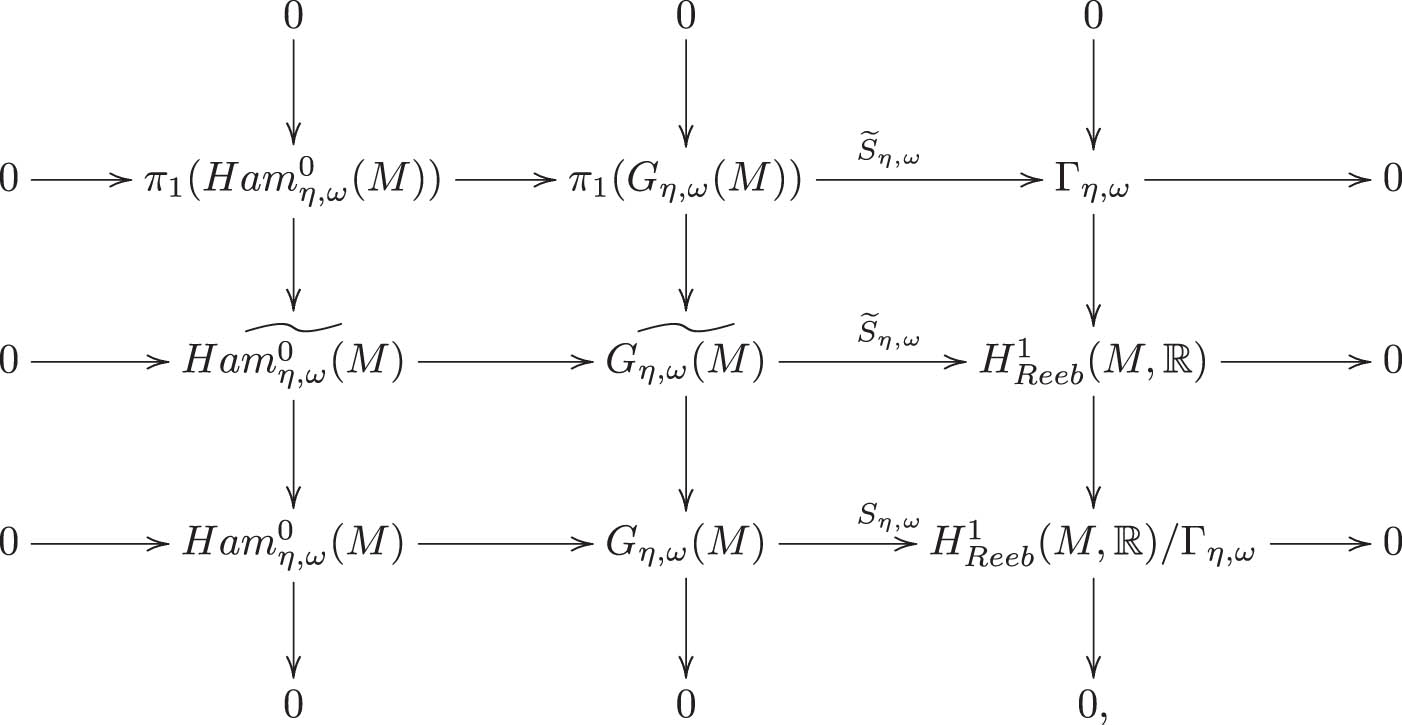
where the first two arrows are incluison mappings.

5 Regularization of co-Hamiltonian paths

Definition 5.1

Let Ψ ≔ { ψ t } be a smooth isotopy. We shall say that Ψ is regular if for every t , the tangent vector to the path Ψ does not vanish.

For this study, we shall need the following subsets:

ℱ ˆ η , ω ( M ) ≔ { F = ( F t ) ∈ C ∞ ( M , R ) : ∫ M F t η ∧ ω n = 0 , ∀ t } : the set of all smooth family of normalized functions on ( M , η , ω ) .
ℱ ˆ ξ ( M ) ≔ { F = ( F t ) ∈ ℱ ˆ η , ω ( M ) : ξ ( F t ) = C t e t , ∀ t } : the set of all smooth family of normalized functions in ℱ ˆ η , ω ( M ) that are constants along the integral curves of the Reeb vector field.
For any element F in ℱ ˆ ξ ( M ) , we shall denote by ψ F the weakly Hamiltonian isotopy generated by F . Let ℱ ˆ ξ 0 ( M ) be the subset of ℱ ˆ ξ ( M ) consisting of elements F such that ξ ( F ) = 0 .

Consider P ˆ ξ ( M ) ≔ { F = ( F t ) ∈ ℱ ˆ ξ 0 ( M ) : F t + 1 = F t , ∀ t } : the set of all smooth family of normalized functions in ℱ ˆ ξ 0 ( M ) that are 1-periodic.
Following the symplectic case, one can show that every co-Hamiltonian diffeomorphism ψ can be represented as the time-1 map of an isotopy generated by an element of P ˆ ξ ( M ) [13]. Furthermore, an isotopy Ψ ≔ { ψ t } generated by an element of P ˆ ξ ( M ) satisfies ψ t + 1 = ψ t ∘ ψ 1 , for all t [13].
Assume that M is closed. Now, pick ψ F ≔ { ψ t } with F ∈ P ˆ ξ ( M ) , and applying Proposition 3.1 to ψ F , we derive that ψ ˜ F is a Hamiltonian isotopy of ( M × S 1 , ω ˜ ) with Hamiltonian function F ˜ t ≔ F t ∘ p , where ω ˜ ≔ p ∗ ( ω ) + p ∗ ( η ) ∧ π 2 ∗ ( d θ ) . Since F t + 1 = F t , for all t , hence F ˜ t + 1 = F ˜ t , for all t . Form ∫ M F t ω n ∧ η = 0 , for each t , we compute
∫ M × S 1 F ˜ t ω ˜ n + 1 = ∫ M × S 1 p ∗ ( F t ω n ∧ η ) ∧ π 2 ∗ ( d θ ) = 2 π ∫ M F t ω n ∧ η = 0 .
Hence, applying a result of Polterovich [13], one obtains the desired result.

Denote by ℒ ˆ ξ ( M ) ≔ { H = ( H t ) ∈ P ˆ ξ ( M ) : ϕ H 1 = id M } . This is the set of all elements in P ˆ ξ ( M ) that generate co-Hamiltonian loops.

Definition 5.2

[13] A k -parameter variation of the constant loop is a smooth family of loops { h t ( ε ) } , where ε belongs to a neighborhood of 0 in R k and h t ( 0 ) = id M for all t . If the manifold M is open we assume in addition that the supports of all h t ( ε ) are contained in some compact subset of M .

Remark 5.3

(Existence of k -parameter variation of the constant loop on ( M , η , ω ) ). Let ( M , η , ω ) be a closed cosymplectic manifold of dimension 2 n + 1 . Pick H ∈ P ˆ ξ ( M ) such that ξ ( H t ) = 0 , for all t , and set G t ≔ H t − ∫ 0 1 H t d t for each t . We have ∫ M H t η ∧ ω n = 0 , for each t , which implies

(5.1) ∫ 0 1 ∫ M H t η ∧ ω n d t = ∫ M ∫ 0 1 H t d t η ∧ ω n = 0 .

Hence, ∫ 0 1 G t ( x ) d t = 0 , for every x ∈ M , ξ ( G t ) = ξ ( H t ) − ∫ 0 1 ξ ( H t ) d t = 0 − 0 , and

(5.2) ∫ M G t η ∧ ω n = ∫ M H t η ∧ ω n − ∫ M ∫ 0 1 H t d t η ∧ ω n = 0 ,

for each t . Furthermore, for each fixed t , the function ∫ 0 t G s d s , generates a co-Hamiltonian flow because ξ ∫ 0 t G s d s = ∫ 0 t ξ ( G s ) d s = 0 . As in [13], define h t ( ε ) ∈ H η , ω 0 ( M ) as the time − ε map of the co-Hamiltonian flow generated by the time-independent Hamiltonian function ∫ 0 t G s d s : If H ( x , t , ε ) is the normalized co-Hamiltonian function generating the flow ( h t ( u ) ) u , then

(5.3) ∂ ∂ ε ∣ ε = 0 H ( x , t , ε ) = G t ( x ) .

Hence, it seems natural to construct k -parameter variations as compositions of 1-parameter variations: h t ( ε 1 , … , ε k ) ≔ h t 1 ( ε 1 ) ∘ ⋯ ∘ h t k ( ε k ) , where each h t j is constructed with the help of a function G j as mentioned earlier so that ∂ ∂ ε j ∣ ε = 0 H ( x , t , ε ) = G t j ( x ) , for each j = 1 , … , k (see [13]).

Proposition 5.4

Let ( ψ t ) be a flow generated by F ∈ ℱ ˆ ξ ( M ) with ξ ( F t ) = 0 , for each t. Then, there exists an arbitrary small co-Hamiltonian loop (in the C ∞ -sense), say ( τ t ) such that the isotopy ( τ t − 1 ∘ ψ t ) is regular.

Proof

With the aid of Remark 5.3, one argues as in the proof of similar result from symplectic geometry (see Proposition 5.2.A-[13]).□

Let us introduce norms on ℱ ˆ η , ω ( M ) as follows. For all F ∈ ℱ ˆ η , ω ( M ) ,

‖ F ‖ ∞ ≔ max t ( max x F ( x , t ) − min x F ( x , t ) ) , and ‖ F ‖ 1 , ∞ = ∫ 0 1 ( max x F ( x , t ) − min x F ( x , t ) ) d t .

Lemma 5.5

Let ( M , η , ω ) be a closed cosymplectic manifold. For all ψ ∈ H a m η , ω 0 ( M ) , we have

ρ Co ∞ ( ψ , id M ) ≔ inf F ∈ ℱ ˆ ξ ( ψ ) ‖ F ‖ ∞ = inf F ∈ ℱ ˆ ξ ( ψ ) ‖ F ‖ 1 , ∞ ≕ ρ Co 1 , ∞ ( ψ , id M ) .

Proof

This is an adaptation of similar result found in the symplectic case [13].□

Here is a consequence of Lemma 5.5.

Lemma 5.6

Let ( M , η , ω ) be a compact connected cosymplectic manifold. Let F ∈ ℱ ˆ ξ ( M ) (fixed), we have ρ Co 1 , ∞ ( ϕ F 1 , id M ) = inf H ∈ P ˆ ξ ( M ) ‖ F − H ‖ ∞ .

Proof

By definition, we have inf H ∈ P ˆ ξ ( M ) ‖ F − H ‖ ∞ ≤ ‖ F ‖ ∞ , which implies

(5.4) inf H ∈ P ˆ ξ ( M ) ‖ F − H ‖ ∞ ≤ ρ Co ∞ ( ψ , id M ) .

On the other hand, ‖ F ‖ ∞ ≤ ‖ F − H ‖ ∞ + ‖ H ‖ ∞ , which implies that

(5.5) ρ Co ∞ ( ψ , id M ) ≤ inf H ∈ P ˆ ξ ( M ) ‖ F − H ‖ ∞ + 0 .

Therefore, the desired result follows from Lemma 5.5.□

6 Locally conformal cosymplectic stability

Definition 6.1

[5] Let M be an odd dimensional manifold equipped with a 2-form ω and a 1-form η such that 2-form I ˜ η , ω ≔ ω + η ⊗ η is non-degenerate on M . Then, M is said to be locally conformal cosymplectic (l.c.c. ) if there exists an open covering { U i } of M and a system of smooth functions f i on each U i such that

(6.1) d ( e 2 f i ω ) = 0 , d ( e f i η ) = 0 .

It is known that the local 1-forms d f i glue up together to a 1-form θ satisfying

(6.2) d ω = − 2 ω ∧ θ , d η = η ∧ θ .

In [5], it is shown that if there is a 1-form satisfying (6.2), then we can obtain a system ( U i , f i ) i satisfying (6.1). The 1-form θ defined in (6.2) is called the Lee form. When the Lee form vanishes identically, the couple of forms ( ω , η ) induces a cosymplectic structure on M . Also, two given l.c.c. structures ( ω , η ) and ( ω ′ , η ′ ) are said to be (conformal) equivalent if there exists a smooth function h such that ω ′ = e h ω and η ′ = e h η .

Furthermore, one can show that the de Rham cohomology class of the Lee forms are invariant of the l.c.c. structure since a conformal rescaling of ω and η changes θ by the addition of an exact form: If two l.c.c. structures ( ω , η ) and ( ω ′ , η ′ ) are conformally equivalent with ω ′ = h ω , and η ′ = h η , then θ ′ = θ + d ( ln h ) .

6.1 Lichnerowicz’ cohomology

Lichnerowicz’ cohomology, also known in the literature as Morse-Novikov cohomology, is a cohomology defined for a smooth manifold M and a closed 1-form α . The Lichnerowicz cohomology is the cohomology of a complex, ( Ω ∗ ( M ) , d α ) , where d α is defined by:

(6.3) d α A = d A − α ∧ A ,

for all A ∈ Ω ∗ ( M ) [9]. Let us assume M to be a smooth manifold, and α a closed 1-form on M . One defines a first-order differential operator d α as follows:

(6.4) d α A = d A − α ∧ A ,

where A is any differential form. It is straightforward to verify that d α squares to zero, so that one obtains a modified de Rham complex ( Ω ∗ ( M ) , d α ) . Its cohomology vector spaces H α ∗ ( M ) are called the d α -cohomology, or Lichnerowicz cohomology of M with respect to α . This only depends on the de Rham cohomology class of α : if α ′ = α − d ln h for some positive function h , then the following relation holds:

(6.5) h d α ′ A = d α ( h A ) .

This shows that multiplication by h is a chain map between ( Ω ∗ ( M ) , d α ) and ( Ω ∗ ( M ) , d α ′ ) inducing an isomorphism in cohomology. If α is the Lee form of a l.c.c. structure ( ω , η ) , then ω and η are d α -closed and so define a class in H α 2 ( M ) and H α 1 ( M ) , respectively. Now, consider the l.c.c. structure defined by ω ′ and η ′ , with ω ′ = f ω and η ′ = f η , then the Lee form of ω ′ and η ′ denoted θ ′ is just θ ′ = θ + d ln f . The class [ ω ] ∈ H α 2 ( M ) is mapped to [ ω ′ ] ∈ H α ′ 2 ( M ) and [ η ] ∈ H α 1 ( M ) is mapped to [ η ′ ] ∈ H α ′ 1 ( M ) by the above isomorphism. It can be found in the literature that Lichnerowicz’ cohomology shares common properties with the usual de Rham cohomology [9].

Theorem 6.2

(Locally conformal cosymplectic stability) Let M be a smooth closed manifold of dimension ( 2 n + 1 ) . Let ( ω t , η t ) be a family of l.c.c. structures with Lee forms θ t depending smoothly on t ∈ [ 0 , 1 ] . There exists an isotopy Φ = { ϕ t } with ϕ t ∗ ( ω t ) and ϕ t ∗ ( η t ) conformally equivalent to ω 0 and η 0 , respectively, for all t, if and only if we can find positive smooth functions h t on M , varying smoothly with t, and such that

∂ ∂ t ( h t ω t ) θ t ′ = [ d θ t ′ α t ] θ t ′ = 0 ,
∂ ∂ t ( h t η t ) θ t ′ = [ d θ t ′ ( L t ) ] θ t ′ = 0 , and
α t ( ξ t ) = 0 ,

where ξ t ≔ I ˜ η t , ω t − 1 ( η t ) , for every t , θ t ′ ≔ θ t + d ln h t is the Lee form w.r.t. h t ω t and h t η t .

Proof

We shall adapt the proof of similar result from symplectic geometry. After a suitable rescaling, we suppose that there exists a smooth isotopy { ϕ t } from M to itself such that ϕ t ∗ ( ω t ) = ω 0 and ϕ t ∗ ( η ) = η , for all t ∈ [ 0 , 1 ] . This tells us that the smooth family of vector fields defined by v t ( ϕ t ( x ) ) ≔ d d t ϕ t ( x ) , for each x ∈ M , satisfies ∂ ∂ t ω t = d θ t ( ι ( v t ) ω t ) + θ t ( v t ) ω t and ∂ ∂ t η t = ( d θ t ( η t ( v t ) ) + θ t ( v t ) η t ) . Now, we set h t ≔ e − ∫ 0 t θ s ( v s ) d s and derive that:

∂ ∂ t ( h t ω t ) = h ˙ t ω t + h t ∂ ∂ t ω t , = − h t θ t ( v t ) ω t + h t ( d θ t ( ι ( v t ) ω t ) + θ t ( v t ) ω t ) , = h t d θ t ( ι ( v t ) ω t ) , = d θ t + d ln h t ( − h t ι ( v t ) ω t ) .

Similarly, we have ∂ ∂ t ( h t η t ) = − d θ + d ln h t ( h t η ( v t ) ) . Taking α t ≔ h t ι ( v t ) ω t , one computes α t ( ξ t ) = h t ω t ( v t , ξ t ) = 0 , for every t . Conversely, first note that in the Lichnerowicz cohomology, the analogue of Hodge theory guarantees that there exists a unique α t (resp. L t ) so that ∂ ∂ t ( ω t ) = d θ t α t and ∂ ∂ t ( η t ) = d θ t L t (if necessary after rescaling ω t and η t ). Consider the family { X t } of vector fields defined as :

(6.6) I ˜ η t , ω t ( X t ) = − α t − L t η t ,

for each t . If Ψ = { ψ t } is the isotopy generated by { X t } , then

d d t ( ψ t ∗ ( η t ) ) = ψ t ∗ ( d ( η t ( X t ) ) + ι ( X t ) d η t + d θ t L t ) , = ψ t ∗ ( d ( η t ( X t ) ) + ι ( X t ) ( θ t ∧ η t ) + d θ t L t ) , = ψ t ∗ ( − d θ t L t + θ t ( X t ) η t + d θ t L t ) , = ψ t ∗ ( θ t ( X t ) η t ) , = ( θ t ( X t ) ∘ ψ t ) ψ t ∗ ( η t ) ,

because (6.6) together with the condition α t ( ξ t ) = 0 , for every t , implies that η t ( X t ) = − L t , for every t . Thus, ψ t ∗ ( η t ) = e ∫ 0 t θ s ( X s ) ∘ ψ s d s η 0 , for all t . Similarly, one shows that ψ t ∗ ( ω t ) = e ∫ 0 t θ s ( X s ) ∘ ψ s d s ω 0 , for all t .□

In the statement of Theorem 6.2, the third condition shows that one cannot avoid the Reeb vector field when studying cosymplectic dynamical systems. Assuming that the Lee forms are time-independent, the above stability theorem implies the following statements.

Corollary 6.3

(Stability A ) Let ( η t , ω t ) be a smooth family of l.c.c. structures on a compact manifold M having the same Lee forms θ . Assume that for each t ∈ [ 0 , 1 ] , I ˜ η t , ω t is an isomorphism over the module C ∞ ( M ) . If ω t = ω 0 + d θ α t , η t = η 0 + d θ L t , and α ˙ t ( ξ t ) = 0 , for all t , with ξ t ≔ I ˜ η t , ω t − 1 ( η t ) , then there exists a family { h t } of functions and an isotopy Φ ≔ { φ t } such that φ t ∗ ( ω t ) = h t ω 0 and φ t ∗ ( η t ) = h t η 0 .

Lemma 6.4

(Stability B ) Let ( η t , ω t ) be a smooth family of l.c.c. structures on a compact manifold M such that the corresponding Lee forms θ t have the same de Rham cohomology class (i.e., θ ˙ t = d h t , for each t ). Suppose there exist smooth families of 1-forms α t and functions L t such that ω t = d α t − θ t ∧ α t , η t = d L t − L t θ t , respectively, and ( h t α t + α ˙ t ) ( ξ t ) = 0 , with ξ t ≔ I ˜ η t , ω t − 1 ( η t ) . Then there exists an isotopy Φ = { φ t } such that φ t ∗ ( ω t ) is conformally equivalent to ω 0 and φ t ∗ ( η t ) is conformally equivalent to η 0 .

Proof

We shall adapt the proof given in [2]. First, we use the fact that the Lee forms θ t have the same de Rham cohomology class to derive that θ ˙ t = d h t . Put, g t ≔ − ∫ 0 t h t , and f t ≔ e g t . As in [2], one shows that

(6.7) ∂ ∂ t ( f t ω ) = d θ t + d ln h t ( f t ( − h t α t + α ˙ t ) ) .

Similarly, one obtains

(6.8) ∂ ∂ t ( f t η ) = d θ t + d ln h t ( f t ( − h t θ t + θ ˙ t ) ) .

Therefore, combining (6.7) and (6.8) together with condition ( h t α t + α ˙ t ) ( ξ t ) = 0 , one applies Theorem 6.2 to conclude.□

Acknowledgments

The author is thankful to the anonymous reviewers for their profound and contribuable comments and to the editor for considering this work. I dedicate this work to the late Dr. Mohamed Kampo who died so soon after defending his Ph.D in mathematics, and faraway from his family : his kindness and his capacity for insight will be forever missed.

Funding information: No funding was received for the accomplishment of this work.
Conflict of interest: The author states no conflict of interest.

References

[1] A. Banyaga, Sur la structure des difféomorphismes qui préservent une forme symplectique, Comment. Math. Helv. 53 (1978), 174–2227. 10.1007/BF02566074Search in Google Scholar

[2] G. Bande and D. Kotschick, Moser stability for locally conformally symplectic structures, Proc. Amer. Math. Sco. 137 (2009), no. 7, 2419–2424. 10.1090/S0002-9939-09-09821-9Search in Google Scholar

[3] L. Buhovsky, Towards the C0-flux conjecture, Algebraic Geometr. Topol. 14 (2014), 3493–3508. 10.2140/agt.2014.14.3493Search in Google Scholar

[4] B. Cappelletti-Montano, A. De Nicola, and I. Yudin, A survey on cosymplectic geometry, Rev. Math. Phys. 25 (2013), no. 10, 1343002. 10.1142/S0129055X13430022Search in Google Scholar

[5] D. Chinea, M. de Leon, and J. C. Marrero, Locally conformal cosymplectic manifolds and time-dependent Hamiltonian systems, Comment. Math. Univ. Carolin. 32 (1991), 383–387. Search in Google Scholar

[6] F. Gallissot, Formes exterieurs en Mécanique, Thèse. Ann. Inst. Fourier 4 (1954), 145–297. 10.5802/aif.49Search in Google Scholar

[7] H. Li, Topology of cosymplectic/cokaehler manifolds, Asian J. Math. 12 (2008), no 4, 527–544. 10.4310/AJM.2008.v12.n4.a7Search in Google Scholar

[8] M. Hirsch, Differential Topology, Graduate Texts in Mathematics, vol. 3, No. 33, Springer Verlag, New York-Heidelberg, 1976; corrected reprint (1994). 10.1007/978-1-4684-9449-5Search in Google Scholar

[9] C. Ida, A note on the basic Lichnerowicz cohomology of transversally locally conformally Kahlerian foliations, Hacettepe J. Math. Stat. 43 (2014), no. 3, 413–423. Search in Google Scholar

[10] M. de Léon and M. Saralegi, Reduction for singular momentum maps, J. Phys. A 26 (1993), no. 19, 5033–5043. 10.1088/0305-4470/26/19/032Search in Google Scholar

[11] P. Libermann, Les automorphismes infinitesimaux symplectiques et des structures de contact, Coll Geom. Diff. Globales Bruxelles (1958), Louvain (1959), pp. 37–59.Search in Google Scholar

[12] A. Lichnerowicz, Coll Geom. Diff., Globales Bruxelles, 1958. Search in Google Scholar

[13] L. Polterovich, The Geometry of the Group of Symplectic Diffeomorphism, Lecture in Mathematics ETH Zü rich, Birkhäuser Verlag, Basel-Boston, 2001. 10.1007/978-3-0348-8299-6Search in Google Scholar

[14] G. de Rham, Form Differentiali et loro integrali, C.I.M.E 2 ciclo, Saltino, Vallombrossa, Agosto, 1960, p. 21. Search in Google Scholar

[15] M. Shafiee, On the relation between cosymplectic and symplectic structures, J. Geom. Phy. 178 (2022), 104–536. 10.1016/j.geomphys.2022.104538Search in Google Scholar

[16] S. Tchuiaga, On symplectic dynamics, Differ. Geom. Appl. 61 (2018), 170–196. 10.1016/j.difgeo.2018.09.003Search in Google Scholar

[17] S. Tchuiaga, F. Houenou, and P. Bikorimana, On cosymplectic dynamics I, Complex Manifolds 9 (2022), 114–137. 10.1515/coma-2021-0132Search in Google Scholar

[18] F. Warner, Foundation of differentiable manifolds and Lie groups, Graduate Texts in Mathematics, vol. 94, Springer-Verlag, New York, 1983. 10.1007/978-1-4757-1799-0Search in Google Scholar

[19] A. Weinstein, Symplectic manifolds and their Lagrangian submanifolds, Adv. Math. 6 (1971), 329–345. 10.1016/0001-8708(71)90020-XSearch in Google Scholar

Received: 2022-11-28

Revised: 2023-05-01

Accepted: 2023-06-16

Published Online: 2023-07-18

This work is licensed under the Creative Commons Attribution 4.0 International License.

Articles in the same Issue

https://doi.org/10.1515/coma-2022-0151

Keywords for this article

Locally conformal cosymplectic manifolds; flux homomorphism; the Weinstein chart; diffeomorphisms; differential forms

Creative Commons

BY 4.0