Mathematical model on influence of past experiences on present activities of human brain
-
P. Raja Sekhara Rao


Abstract
This article explores how emotional feelings linked to stored memories of past experiences influence the present activity of the human brain. To analyse this, a mathematical model is considered describing the dynamics in a two-layered network in which the neurons in the first layer are involved in present activities and are influenced by cells in the second layer that carry the emotional feelings associated with memories of past experiences. Initially, this article establishes sufficient conditions for the stability of a unique equilibrium solution in the system for both constant and time-varying exogenous inputs. This indicates the situation where the present activities are not disturbed by emotions emanated from past memories. Furthermore, it is observed that certain variations in the exogenous inputs can induce oscillations within the system. To manage them, this study suggests the adjustment of specific parameters that could actually control certain fluctuations according to emotional responses to past and current memories. This control aims to stabilize the brain’s current activity, allowing it to reach a balanced state.
1 Introduction
Human beings are emotional, and their activities are usually emotion driven. One knows that emotions are generated by experiences. If the experiences are not in the physical world, the brain has the ability to get the same in an imagined world. Our feelings towards crime news, expected exam results, the performance of our football team in tomorrow’s match, pandemics like Covid-19 – all are imagined, stored with some emotions or impressions that may be recalled or come into the forefront when the actual situation arises. Furthermore, the emotions of a person have an impact on the surroundings or society [24]. Thus, the study of the influence of emotions is interesting and useful. Based on one’s emotions, we may predict one’s behaviour to some extent. Emotions are reflected through facial expressions or other body gestures. Scientists have been studying extensively to predict emotions and consequent actions by analysing physical body gestures. Many researchers from different fields such as social sciences, biological sciences, mathematical sciences, and engineering sciences are working on the role of emotions in their perspective. Psychologists have focused on the psychological aspects of the cause and impact of these emotions. Many emotional theories have been described by them to predict or recognize the emotions of a person. Biologists have studied the contribution of the activities of the brain on emotions and their responses. Computer scientists have tried to predict or recognize emotions using artificial neural networks. Mathematicians have tried to frame a mathematical model for emotions using different approaches.
In psychology, according to the classical view of emotion, emotions can be assessed objectively and accurately through facial expressions. But how does the brain guide us for a particular action for different emotions based on the situations? This is a key point on which many researchers are working. Barrett [3] and Zimmerman [27,28] have said that these actions for emotions are generated by the brain by using the concepts stored in the memory by earlier experiences. Albarracin [1] stated that a person’s attitudes and behaviour will be influenced by their past experience and past behaviour. Hartmann et al. have used appraisal theory to predict emotions by forming a mathematical model for emotions [7]. Islam et al. have modelled the emotional states based on wavelet analysis and the trust-region algorithm, which can be applied to hardware implementation of human emotion-based systems [9]. Prisnyakov and Prisnyakova have expressed human adaptation to emotional factors by using a model of information processing by memory [15]. Ambrosio [2] provided a mathematical approach to characterize the emergence of emotional fluxes in the human psyche. Iinuma and Kogiso [8] proposed a computational human decision-making model that handles emotion-induced behaviour. Gupta et al. [6] have tried to simulate and model the human decision-making process through a reinforcement learning-based computational model involving past experiences.
Now coming to the study of emotions using a neural network. Levine et al. [11] have performed a detailed discussion on different types of neural network models available in the literature for different types of emotions. Lee et al. [10] have used a neural network to recognize emotions through heart rate variability and skin resistance. Unluturk et al. [25] studied emotions using speech recognition by introducing a new type of neural network called ERNN. Thenius et al. [23] have proposed a new type of neural network named EMANN to predict emotions. Sharma and Dugar [22] have tried to recognize emotions through face detection using deep neural networks. Minaee and Abdolrashidi [14] have predicted emotions through facial expressions by using attentional convolutional networks. Rahul Mahadeo Shahane and Ramakrishna Sharma [16] have used a feed-forward neural network to recognize emotions. Santhoshkumar and Geetha [21] have used feed-forward deep convolution neural networks for emotion recognition from human body movements. Merlin et al. [13] have studied and compared different approaches to identify emotions on human faces, considering multiple perspectives on emotion detection by using the Viola-Jones face detection method to identify faces. Manalu and Rifai [12] used hybrid convolutional neural network-recurrent neural network algorithm to detect human emotions through facial expressions. Begazo et al. [4] have tried to detect human emotions through voice using deep learning techniques. We can see most of the work is to predict or recognize emotions, which has a wide application in the fields of marketing, economic theory, banking, the hospitality industry, media and communication, etc. Thus, so far, studies have appeared to focus on understanding which emotion caused the activity.
Our aim in this article is to understand the converse, i.e., how emotions from stored experiences could influence other activities of the human brain. This we try to do in a mathematical way! Explaining the complex phenomena of the human brain through mathematical equations is not an ordinary task. However, attempts are made to enter this labyrinth in some way, somehow, to begin with. To our knowledge, there are two ways to go. Consider as many phenomena of the brain as possible and put them in the form of mathematical equations, solve them, and see how far the solutions explain the phenomena, and modify equations, if necessary, to fit them best. This is going to be an ominous task as far as a highly complex system such as the human brain is concerned. The second path is a simpler one: select an existing mathematical model, and check how far it explains the features of the system under consideration. Modifications are always possible in a mathematical model to make it suitable for the system. This prompts us to consider the model proposed by Rao and Rao [20]. The model was proposed to study the interactive dynamics between two layers of a network of nodes (components or neuronal cells) that describe a hierarchical system, such as an information management system. We are going to utilize this model to see how emotional feelings emanating from past experiences or recorded memories influence the activities of the brain.
Except for natural activities such as attending to basic physical needs, and knee-jerk reactions, all activities of the brain involve both thinking and recalling. Thinking may be regarded as an activity of the brain for the situation under consideration, while recalling is an activity of the brain with regard to its previous experiences stored in memory, along with some impressions or attributes. A single experience could be a result of many activities, and one activity may be the root cause of many memories. Thus, each neuron in one layer could be attached to one or more neurons in another layer. In other words, certain interactive dynamics are created between these two activities of the brain. How to represent this?
For this, we consider two layers of neurons:
The first layer consists of neuronal cells that are involved in the present activities, and the second layer consists of those neuronal cells that reflect the emotional feelings attached to memories of past experiences.
Each neuron in the first layer is connected to a set of neurons (specific to it) in the second layer that tends to influence it through related memories. Thus, both layers are interconnected.
All neurons in both the layers are intra-connected among themselves.
An input to the brain will stimulate both layers of neurons. In other words, inputs to the system invoke activity in the first layer as well as stimulate activity in memory cells in the second layer.
for
where
The response functions
In [20], it is assumed that neurons in the first layer are always supported by neurons in the second layer and, hence, are termed as cooperative and supportive network. In this article, we are going to understand how the sub-network neurons are going to influence the activities of main network neurons and how these influences are withstood to carry out their activities. Thus, the neurons
How do the dynamics of stored memories influence the related activities of the brain?
How to work along with emotions in parallel?
Can the system remain stable under fluctuating emotions?
This article is organized as follows. In Section 2, a modified form of (1) is presented that includes all possible delays in communication and transmission of data in such networks. Basic properties such as the existence and uniqueness of solutions and also equilibria are discussed. Section 3 deals with the stability properties of solutions of the system considered under the influence of both constant inputs and time-varying inputs. Several sufficient conditions are obtained via Lyapunov functionals. In Section 4, we provide illustrative examples to verify the results of Section 3 and try to answer the questions posed earlier. A discussion concludes the work in Section 5.
2 Model and basic properties
The brain always learns and adds experiences from present activities into the memory store while working simultaneously with them. We consider this ability of the brain and introduce the corresponding term into (1). Concurrency of many activities at the same time may lead to processing delays among
for
where all the terms remain as defined in (1). Here, the new terms
The pictorial representation of this network may be depicted in Figure 1.
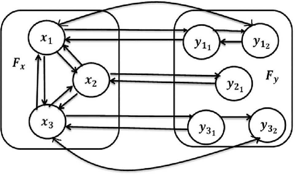
Typical representation of the proposed network. Source: Created by the authors.
By the theory of delay differential equations, we know that the local Lipschitz conditions on response functions guarantee the existence of solutions. Hence, we assume the following Lipschitz conditions on the response functions:
for some positive constants
In view of conditions (3), we assume henceforth that the system (2) possesses unique solutions that are continuous in their maximal intervals of existence. The response functions
The most common way of understanding the dynamics of a system, such as (2), is to study its behaviour at equilibrium solutions in terms of its stability. An equilibrium solution represents a known constant solution of the system, and convergence to such a known value implies that the activities are concluding to a known action/solution. An autonomous system such as (2) may possess equilibria. Existence of equilibria remains unaffected by time delays, as demonstrated in previous studies [5,17,19,20]. Therefore, we can establish that
Theorem 2.1
If the output functions satisfy conditions (3) and the parameters satisfy conditions
then model (2) has a unique equilibrium solution.
Thus, under conditions (4), model (2) possess a unique equilibrium, which may typically be represented by
where
We will be using equations (5) whenever required in our results.
Now the question arises, under what conditions on the system parameters and functional responses do the solutions of model (2) converge to an equilibrium solution? In the next section, we try to establish different sets of sufficient conditions for the solutions to reach the equilibria reflecting the asymptotic stability of the system.
3 Stability aspects
We directly start with the stability of the unique equilibrium of (2) that exists by virtue of Theorem 2.1. The following result provides sufficient conditions on the system parameters for global asymptotic stability of equilibrium solution of (2).
Theorem 3.1
Assume that conditions (3) hold. If
for all
Proof
By choosing
the upper Dini derivative of
where
By hypothesis,
Conclusion follows from the standard argument.□
Remark 3.2
What does the stability of an equilibrium in such activities mean? For mathematicians, an equilibrium point is a stationary or critical point where the system is in a resting state. For activities linked to a brain or an artificial neural network, an equilibrium point is regarded as (stored) memory pattern or state where the brain/network exhibits no dynamics. Thus, it represents a state of calmness, and the brain has come to a conclusion or is focused. Theorem 3.1 provides sufficient conditions (
We shall now provide some more sets of conditions on parameters for global asymptotic stability of model (2). The following inequality enables us to find more general conditions on the parameters of the system for the global asymptotic stability of equilibrium solution.
For all real numbers
holds true.
Theorem 3.3
Assume that conditions (3) hold. The equilibrium
Proof
(a) We construct the appropriate Lyapunov functional.
We consider
Differentiating
Using (8) for
Substituting (10) into (9), we obtain
Let
Then, the derivative of
Using (8) for
Substituting (13) into (12), we obtain
Now, consider the functional
Now, let
Then, the time derivative of
where
for
By hypothesis
We now consider case (b)
(b) As in earlier case, we consider the functional
For
Substituting (16) into (9) and simplifying, we obtain
Proceeding as in
The remainder of the proof is the same as that of earlier cases
Remark 3.4
Theorem 3.3 presents several sets of sufficient conditions on the parameters and functionals of the model. This means that model (2) has a larger region of stability and, thus, could provide a reasonable solution with suitable inputs. Such systems exhibit a tendency to stay stable, calm or said to have a focused state of mind and can work synchronously with past experiences for executing present activity in a better way.
Remark 3.5
One may note that for
It may be noted that none of the conditions in Theorems 3.1–3.3 depend on the delay parameters. Hence, these results are valid for all delays and, in particular, when
3.1 Time-varying inputs
In artificial neural networks, fluctuations in input current, voltage, noise, etc., lead to variable inputs to the system. Human brain receives many inputs from the sense organs of the body besides internal inputs from stored data. Bringing exact input to recall a particular memory is rarely possible for a complex system as a brain. A continuous process of inputs that triggers the thought process that leads to the desired output is our usual experience. Thus, inputs to a system need not always be fixed constants. On the other hand, when multiple activities are carried out simultaneously, the inputs of one activity may interfere with the other. Such inputs are capable of disturbing the system, sometimes leading the system to nowhere. It is our common experience that when similar activities are going on in our brain, inputs to one activity may be mistakenly attributed to another activity, leading to wrong conclusions – what we call a confused state of mind. These observations motivate us to study the impact of changing inputs. Since uncontrolled inputs lead to uncontrolled systems, we restrict our study to the following cases: (i) inputs to both present activities and past experiences converging or approaching some fixed values; (ii) one of the inputs is fluctuating – reflecting an oscillatory-type input, and the other is converging to a finite value; and (iii) both types of inputs are oscillatory, reflecting a wavering mind. In the first case, one may expect the system to behave well in the sense that the solutions approach some fixed state, as in the case of constant inputs. The same is established by means of a result here. In the latter two cases, one may expect a fluctuating mind drawing no fixed conclusions, inferring a non-focused state of mind. Then, we propose some mechanisms that could possibly control these fluctuations introduced by variable inputs. We explain this through illustrative examples.
With this background, we shall now let the exogenous inputs
where
Under the conditions (3) on response functions, appropriate initial conditions and assuming the inputs
Our known model is (2), and we have considered model (18). With all the parameters and functional relations being the same, the only difference between the two systems is between the inputs. One natural question could be, will the solutions of (2) and (18) behave closely or similarly if the corresponding inputs stay close enough? The following result establishes this. That means we try to restrict the inputs of (18) for which the solutions of model (18) will converge to the solutions of model (2), implying that both systems behave closely or similarly eventually.
Theorem 3.6
Assume that the parametric conditions (6) hold for model (18), let the inputs satisfy
Proof
Consider
Taking the Dini derivative along the solutions of model (18):
where
Integrating from 0 to t, we obtain
given
So, the aforementioned inequality implies that
But we know even
Hence, we can conclude that
Corollary 3.7
Assume that all the hypotheses of the
Theorem 3.6
are satisfied. Furthermore, if model (2)possesses equilibrium pattern
Proof
The result follows from the observation that the equilibrium solution
Remark 3.8
By taking the parameter
Furthermore, by letting
Remark 3.9
External inputs to a system always influence the dynamics of the system. They decide the equilibria of the system and their stability and may even make the system unpredictable. Thus, tolerable limits are to be obtained for variations in inputs for which the system is not distorted. Model (2) is well behaved in the sense of Theorems 3.1–3.3, and it approaches a predictable (equilibrium) state. On the other hand, model (18) does not possess equilibria. Then, how to study its behaviour, or where does it go? It may be regarded as a simple distortion of model (2) as the only difference between them is in terms of their inputs. Thus, a reasonable way to study its behaviour is to examine its solutions could be with respect to those of system (2), of which one solution is its equilibrium state. This means that if the solutions of model (18) are also approaching the equilibrium
From the aforementioned result, it is noted that if the inputs satisfy the conditions of Theorem 3.6, then the behaviour of solutions of the model with time-varying inputs (18) is similar to that of solutions of the model with constant inputs (2).
In the next section, we provide a variety of situations in the form of numerical examples to illustrate the aforementioned results.
4 Examples and simulations
To understand the behaviour of the system with constant and time-varying inputs, we present two systems, beginning with a simple system with one neuron in each layer and next a system with two neurons in the first layer supported by two neurons each in the second layer. We allow different transmission functions (
Example 4.1
In the aforementioned system, we let
Case (i) For

(a)–(d) are the solution profiles of system (19) with constant inputs for different functions of
We now consider system (2) (or (18)), as the case may be, with two neurons in the first layer, which, in turn, are connected to two neurons each in the second layer.
Example 4.2
Here, we assume that
Case (i). Let
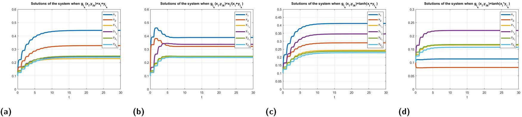
(a)–(d) are the solution profiles of system (20) with constant inputs for different functions of
The following cases illustrate the impact of variable inputs under the auspices of Theorem 3.6 for the systems considered in the aforementioned examples.
Case (ii)(a) Consider

(a)–(d) are the solution profiles of system (19) for different interaction functions with time-varying inputs satisfying the constraints of Theorem Theorem 3.6. System is able to recall the same memories under such disturbances that are eventually coming closer to fixed ones. Source: Created by the authors. Matlab has been used to plot the graphs.
Case (ii)(b) Consider

(a)–(d) are the solution profiles of the system (20) for various interaction functions with time-varying inputs satisfying the constraints of Theorem 3.6. The multi-neuron system demonstrates the ability to retrieve related memories despite the occurrence of disturbances due to control inputs. Source: Created by the authors. Matlab has been used to plot the graphs.
Case (iii) (a) Consider

(a)–(d) are the solution profiles of system (19) with distinct interactive functions, where inputs
Case (iii) (b) Now consider

(a)–(d) are the solution profiles of system (20) for different interaction functions with oscillation inputs
In the aforementioned case, the oscillations that arose in
Case (iv)(a) Let

(a)–(d) are the solution profiles of the system (19) of Case (iii)(a) for various interaction functions with interaction parameter
Case (iv)(b) Let

(a)–(d) are the solution profiles of the system (20) of Case (iii)(b) for distinct functions of
Case (v)(a) Assuming

(a)–(d) are the solution profiles of the system (19) of Case (iii)(a) for various interaction functions with interaction parameter as
Case (v)(b) For

(a)–(d) are the solution profiles of the system (20) of Case (iii)(b) for different functions of
Case (vi)(a) Now we consider the case where the inputs to past experiences are oscillatory, while inputs to the present state are time-varying but not fluctuating, i.e., we let
(a)–(d) are the solution profiles of the system (19) for various interaction functions, where input
Case (vi)(b) Consider

(a)–(d) are the solution profiles of the system (20) with different functions of
As
Case (vii)(a) We let

(a)–(d) are the solution profiles of the system (19) in Case (vi)(a) for different interactive functions with
Case (vii)(b) In this case, we assume

(a)–(d) are the solution profiles of the system (20) in Case (vi)(b) for various interactive functions with smaller values of interaction function
Case (viii)(a) Now let

(a)–(d) are the solution profiles of the system (19) in Case (vi)(a) for various interactive functions with
Case (viii)(b) In case of system (19), we let
(a)–(d) are the solution profiles of the system (20) in Case (vi)(b) for various functions of
The following are the cases where both present and past experiences are triggered by oscillating inputs.
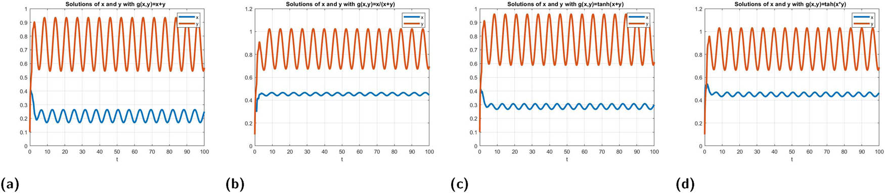
Case (ix)(a) We choose

(a)–(d) are the solution profiles of the system (19) for various interaction functions with oscillatory inputs. The system exhibits oscillations, showing that the brain’s activities may not be stable when the inputs from past and present emotions fluctuate. Source: Created by the authors. Matlab has been used to plot the graphs.
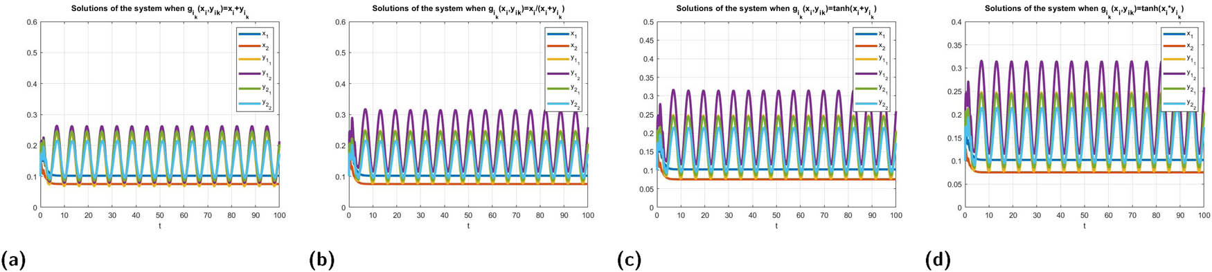
Case (ix)(b) For (19), we let

(a)–(d) are the solution profiles of the system (20) for distinct interactive functions with oscillatory inputs. The fluctuating inputs from both past and present memories influence the activities of the brain. Source: Created by the authors. Matlab has been used to plot the graphs.
Observations:
From the aforementioned two examples, we note the following:
If
The oscillations of
If
In view of the aforementioned observation, the influence of
If both inputs are not within the constraints of Theorem 3.6, then both
| Case | External inputs | Observations | Simulations |
|---|---|---|---|
| (i) |
|
Both
|
Figures 2 and 3 |
| (ii) |
|
Both
|
Figures 4 and 5 |
| (iii) |
|
|
Figures 6 and 7 |
| (iv) | In view of Case (iii), the rate of interaction
|
Oscillations in
|
Figures 8 and 9 |
| (v) | In view of Case (iii), the rate of interaction
|
No more oscillations in
|
Figures 10 and 11 |
| (vi) |
|
|
Figures 12 and 13 |
| (vii) | In view of Case (vi), transmission rate
|
Oscillations in
|
Figures 14 and 15 |
| (viii) | In view of Case (vi), transmission rate
|
|
Figures 16 and 17 |
| (ix) | Both
|
Both
|
Figures 18 and 19 |
Remark 4.3
From the aforementioned observations, the present activities of the brain obtain disturbed in two ways: (i) when the time-varying external inputs influence it and (ii) when the fluctuations invoked by
Similarly, it may also be observed that fluctuations generated by time-varying external input
So far, we have studied the impact of external time-varying inputs and noted that they are capable of disturbing the activities of the system. It is well known in the literature that time delays have the capacity to destabilize a system characterized by oscillations during transition. But Theorems 3.1–3.3 establish global stability of model (2), and the sufficient conditions are independent of time delays also. This implies that the system is less influenced by time delays in the parametric spaces defined by them. We shall explore through numerical examples to see if delays have any impact when the conditions of the aforementioned theorems fail to hold. Since processing delays are very small and negligible in such systems, we consider only transmission delays here.
Let us examine two numerical systems, each of which contains two neurons in the first layer. In one system, these neurons are supported by one neuron each in the second layer, while in the other system, they are supported by two neurons each in the second layer.
Example 4.4
where
Example 4.5
where
Both systems (21) and (22) do not satisfy any parametric conditions of Theorems 3.1–3.3. Yet the simulations of systems (21) and (22), which can be seen in Figure 20(a) and (b), respectively, show that the model is stable in the long run.
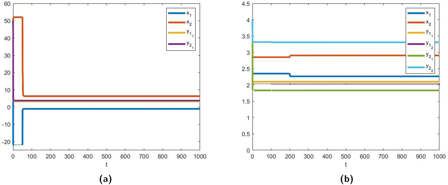
Remark 4.6
It is evident from the aforementioned illustrations that model (2) is not losing its stability even for large values of time delays, which means that time delays have little impact on it. Furthermore, the parametric conditions of our results are only sufficient but not necessary. Hence, it may be inferred that model (2) exhibits strong stability characteristics and has a larger stability region than estimated by Theorems 3.1 and 3.3.
5 Discussion
In this article, an attempt is made to understand the impact of emotional feelings that arise from stored memories of past experiences on the related activities of the human brain. A mathematical model existing in the literature is considered and modified to explain this phenomenon. When the inputs to the system are constant, sufficient conditions on system parameters and functions are obtained to keep the system stable and approach asymptotically an equilibrium solution. Thus, activities of the brain are carried out without hindrance here. Unless thought processes conclude, the brain cannot give commands or take decisions to carry out any activity. Such conclusions are studied as stability of steady states, which are fixed solutions of the system.
Introducing time-varying inputs to the system, (A) it is established that as long as the inputs are within a given range from their constant counterparts, the solutions of the system remain close to the solutions of the corresponding system with constant inputs, and the solutions approach the same equilibrium solution of the system with constant inputs (Theorem 3.6). The system remains stable under damped oscillations as well. (B) When the inputs are beyond the range specified by Theorem 3.6, oscillations are noted, indicating that emotions do have an impact on the activities of the brain, and vice versa. Such situations may be handled by reducing the impact of interaction parameters (
In order to explore the possibilities of a Hopf bifurcation, we have tried large values of transmission delays, but our illustrations reflect that there is little impact of transmission delays on the system. We have not considered processing delays here as they are usually very small in systems such as (2), and choosing large values for them makes it unrealistic. Though we have considered the violation of parametric conditions of Theorems 3.1 and 3.3, the system appears to be stable. This stability looks strong and suggests that the stability regions estimated here are only a small part of the large stability region of model (2). Thus, further exploration of the stability regions of model (2) is welcome.
We feel that the present content may be applicable to improve the performance or output of search engines on the internet where input search words given (
Any mathematical model becomes realistic if it withstands some test data and proves to be useful. At present, the authors are content with establishing theoretical results and explaining some phenomena of the brain. At the same time, testing of a theoretical model with real-time data may lead to the modification of the model and reinterpretation of its parameters or functional relations. For the present context, testing of our models with test data is deferred to a future exposition.
Acknowledgments
The authors are thankful to anonymous reviewers for their stimulating comments that led to a better presentation of the material.
-
Funding information: This research work was carried out without a specific grant from any funding agency.
-
Author contributions: P. Raja Sekhara Rao: Methodology, interpretation of results and manuscript writing. K. Venkata Ratnam: Conceptualization, simulations of numerical examples, manuscript editing, and formatting. G. Shirisha: Literature review, derivations of results, simulations of numerical examples and manuscript writing. All authors reviewed and approved the final version of the manuscript.
-
Conflict of interest: All authors declare that they have no conflict of interest.
-
Ethical approval: This research did not involve any human participants or animals. Ethical approval was therefore not required.
-
Data availability statement: Data sharing is not applicable to this article as no new datasets were generated or analysed during the current study.
References
[1] Albarracin, D. (2021). Chapter 5 - The Impact of Past Experience and Past Behavior on Attitudes and Behavior, (pp. 129–157), Cambridge University Press, Cambridge. DOI: 10.1017/9781108878357.006. Search in Google Scholar
[2] Ambrosio, B. (2020). Beyond the brain: towards a mathematical modeling of emotions. Journal of Physics: Conference Series. 2090, 012119. DOI: 10.1088/1742-6596/2090/1/012119. Search in Google Scholar
[3] Barrett, L. F. (2017). How emotions are made: The secret life of the brain. Boston: Houghton Mifflin Harcourt. Search in Google Scholar
[4] Begazo, R., Aguilera, A., Dongo, I., & Cardinale, Y. (2024). A combined cnn architecture for speech emotion recognition. Sensors, 24, 5797. DOI: 10.3390/s24175797. Search in Google Scholar PubMed PubMed Central
[5] Shirisha, G., & Venkata Ratnam, K. (2022). Dynamical behavior of cooperative supportive system involving intra-network delays in information propagation. Journal of Applied Nonlinear Dynamics, 11, 719–739. DOI: 10.5890/JAND.2022.09.012. Search in Google Scholar
[6] Gupta, N., Ahirwal, M., & Atulkar, M. (2022). Simulation and modeling of human decision-making process through reinforcement learning based computational model involving past experiences. Decision Science Letters, 11, 366–378. DOI: 10.5267/j.dsl.2022.9.001.Search in Google Scholar
[7] Hartmann, K., Siegert, I., Glüge, S., Wendemuth, A., Kotzyba, M., & Deml, B. (2012). Describing human emotions through mathematical modelling. IFAC Proceedings Volumes, 45, 463–468. DOI: 10.3182/20120215-3-AT-3016.00081. Search in Google Scholar
[8] Iinuma, K., & Kogiso, K. (2021). Emotion-involved human decision-making model. Mathematical and Computer Modelling of Dynamical Systems, 27, 543–561. DOI: 10.1080/13873954.2021.1986846. Search in Google Scholar
[9] Islam, M., Ahmad, M., Yusuf, M. S. U., & Ahmed, T. (2015). Mathematical modeling of human emotions using sub-band coefficients of wavelet analysis. 2015 International Conference on Electrical Engineering and Information Communication Technology (ICEEICT), (pp. 1–6). DOI: 10.1109/ICEEICT.2015.7307398. Search in Google Scholar
[10] Lee, C., Yoo, S. K., Park, Y., Kim, N., Jeong, K., & Lee, B. (2005). Using neural network to recognize human emotions from heart rate variability and skin resistance. 2005 IEEE Engineering in Medicine and Biology 27th Annual Conference, 2005, 5523–5525. DOI: 10.1109/IEMBS.2005.1615734. Search in Google Scholar PubMed
[11] Levine, D. S. (2007). Neural network modeling of emotion. Physics of Life Reviews, 4, 37–63. DOI: 10.1016/j.plrev.2006.10.001. Search in Google Scholar
[12] Manalu, H. V., & Rifai, A. P. (2024). Detection of human emotions through facial expressions using hybrid convolutional neural network-recurrent neural network algorithm. Intell. Syst. Appl., 21, 200339. DOI: 10.1016/j.iswa.2024.200339. Search in Google Scholar
[13] Merlin, C. D., Ravi, V. R., Parthiban, M, Yashwanth Raj A, Mohanasundaram M, & Sathish, A. (2024). Human behavioural identification in different aspects using neural network. 2024 7th International Conference on Circuit Power and Computing Technologies (ICCPCT), 1, 570–575. DOI: 10.1109/ICCPCT61902.2024.10672662. Search in Google Scholar
[14] Minaee, S., & Abdolrashidi, A. (2019). Deep-emotion: Facial expression recognition using attentional convolutional network, Sensors (Basel, Switzerland), 21, 3046. DOI: 10.3390/s21093046. Search in Google Scholar PubMed PubMed Central
[15] Prisnyakov, V., & Prisnyakova, L. (1994). Mathematical modeling of emotions. Cybernetics and Systems Analysis, 30, 142–149. DOI: 10.1007/BF02366374. Search in Google Scholar
[16] Rahul Mahadeo, S., Sharma, R., & Siddeeq, S. (2019). Emotion recognition using feed forward neural network and naive bayes. International Journal of Innovative Technology and Exploring Engineering, 9, 2487–2491. DOI: 10.35940/ijitee.B7070.129219. Search in Google Scholar
[17] Raja Sekhara Rao, P., Venkata Ratnam, K., Ponnada, L., & Satpathi, D. (2017). Global dynamics of a cooperative and supportive network system with subnetwork deactivation. Nonlinear Dynamics and Systems Theory, 17, 205–216. https://www.e-ndst.kiev.ua/v17n2/8(59).Search in Google Scholar
[18] Rao, P. R. S., Ratnam, K. V., & Lalitha, P. (2014). Estimation of inputs for a desired output of a cooperative and supportive neural network. International Journal of Emerging Technologies in Computational and Applied Sciences, 9(1), 99–105. https://api.semanticscholar.org/CorpusID:15908105. Search in Google Scholar
[19] Rao, P. R. S., Ratnam, K. V., & Lalitha, P. (2015). Delay independent stability of co-operative and supportive neural networks. Nonlinear Dynamics and Systems Theory, 15, 184–197. https://www.e-ndst.kiev.ua/v15n2/7(51).Search in Google Scholar
[20] Rao, V. S. H., & Rao, P. R. S. (2007). Cooperative and supportive neural networks. Physics Letters A, 371, 101–110. DOI: 10.1016/j.physleta.2007.06.049. Search in Google Scholar
[21] Santhoshkumar, R., & Geetha, M. K. (2019). Deep learning approach for emotion recognition from human body movements with feedforward deep convolution neural networks. Procedia Computer Science, 152, 158–165. DOI: 10.1016/j.procs.2019.05.038. Search in Google Scholar
[22] Sharma, J., & Dugar, Y. (2018). Detection and recognition of human emotion using neural network. International Journal of Applied Engineering Research, 13, 6472–6477. https://api.semanticscholar.org/CorpusID:201821476.Search in Google Scholar
[23] Thenius, R., Zahadat, P., & Schmickl, T. (2013). Emann - a model of emotions in an artificial neural network. In: Proceedings of the ECAL 2013: The Twelfth European Conference on Artificial Life. ECAL 2013 (pp. 830–837). Sicily, Italy: ASME. DOI: 10.7551/978-0-262-31709-2-ch122. Search in Google Scholar
[24] Trampe, D., Quoidbach, J., & Taquet, M. (2015). Emotions in everyday life. PLoS ONE, 10, e0145450. DOI: 10.1371/journal.pone.0145450. Search in Google Scholar PubMed PubMed Central
[25] Unluturk, M. S., Oguz, K., & Atay, C. (2009). Emotion recognition using neural networks. In: Proceedings of the 10th WSEAS International Conference on Neural Networks. (pp. 82–85). Prague, Czech Republic: World Scientific and Engineering Academy and Society (WSEAS).Search in Google Scholar
[26] Vadrevu, S. H. R., & Rao, P. (2016). Time varying stimulations in simple neural networks and convergence to desired outputs. Differential Equations and Dynamical Systems, 26, 81–104. DOI: 10.1007/s12591-016-0312-z. Search in Google Scholar
[27] Zimmerman, P, “How emotions are made,” Noldus. Accessed: May 11, 2023. [Online]. Available: https://noldus.com/blog/how-emotions-are-made.Search in Google Scholar
[28] Zimmerman, P, “How to measure emotions,” Noldus. Accessed: June 23, 2023. [Online]. Available: https://noldus.com/blog/how-to-measure-emotions.Search in Google Scholar
© 2025 the author(s), published by De Gruyter
This work is licensed under the Creative Commons Attribution 4.0 International License.
Articles in the same Issue
- Special Issue: Differential Equations and Control Problems - Part II
- Mathematical model on influence of past experiences on present activities of human brain
- Special Issue: Data-driven Modeling
- Simulation study on the impact of measurement errors in hierarchical Bayesian semi-parametric models
- Research Articles
- Understanding biofilm--phage interactions in cystic fibrosis patients using mathematical frameworks
- Existence and uniqueness of solution for a fractional hepatitis B model
- Mathematical model of the impact of chemotherapy and antiangiogenic therapy on drug resistance in glioma growth
- Study of transmission pattern of COVID-19 among cardiac and noncardiac population using a nonlinear mathematical model
- Analysis of a fractional-order prey-predator model with prey refuge and predator harvest using the consumption number: Holling type III functional response
- Analysis of a fractional-order model for acute and chronic hepatitis-B transmission with Mittag-Leffler kernels
- Tumor dynamics model with treatments by oncolytic virotherapy and MEK inhibitors involving TNF-α inhibitors: Stability analysis and optimal control