Anisotropic Adaptive Finite Elements for a p-Laplacian Problem
-
Paride Passelli
 and
Marco Picasso
and
Marco Picasso


Abstract
The p-Laplacian problem
1 Introduction
Adaptive meshes demonstrated their efficiency to solve PDEs at a reduced computational cost, for a given level of accuracy. When boundary or internal layers are involved, anisotropic meshes, that are meshes with large aspect ratio, should be considered [24, 3]. The adaptive criteria is, when possible, based on an a posteriori error estimates, see for instance [1, 4, 6, 18, 40, 47, 49] in the isotropic framework and [9, 10, 16, 21, 22, 23, 27, 35, 36, 39, 42, 43, 50] when anisotropic meshes are considered.
A posteriori error estimates for the p-Laplacian problem
In this paper the model problem is studied with anisotropic finite elements. Since the anisotropic meshes are not nested, the framework of [8, 17] cannot be used. A residual-based anisotropic error estimator is derived for the p-Laplacian problem and an anisotropic adaptive algorithm is presented. We show that the error estimator is equivalent to the error in a quasi-norm, up to higher order terms. The involved constants are independent of μ, the solution, the mesh size and aspect ratio. We derive an upper bound for the classical
The outline is the following: in Section 2 the problem and the numerical method are presented. In Section 3, we introduce the anisotropic finite element setting and Clément interpolation estimates in
2 Problem Statement and Numerical Method
Consider a polygonal domain
where
When
To solve problem (2.2), we use classical continuous piecewise linear finite elements. Consider, for any
Existence and uniqueness of
3 Anisotropic Finite Elements and Clément’s Interpolation Estimates
Anisotropic finite elements, that is meshes with possibly large aspect ratio, are considered.
The framework of [22, 23] is used. For any
where
and
In the above notations, for a given
For each K, the cardinality of
For each K, the diameter of
Both assumptions guarantee that the constants involved in the interpolation estimates are mesh aspect ratio independent, which is necessary when working with anisotropic meshes. In particular, the second assumption excludes too distorted reference patches, an example of acceptable and non-acceptable patch is presented in Figure 1.
The two assumptions seem to be fulfilled when using the anisotropic mesh generators in our numerical experiment [22, 23, 38, 43]. The Clément’s interpolant [15] is an important tool for deriving residual based a posteriori error estimates in the

Top: example of acceptable patch: the size of
Let
Proposition 1 (Anisotropic Clément Interpolation Error Estimate in the
L
p
Norm).
For
where
Proof.
Let
Using the equivalence between the p-norm and the 2-norm in
After the change of variable (3.1), since
Moreover,
Using (3.4), we therefore obtain
Proceeding in a similar way we have for
Using again (3.4), we obtain
which concludes the proof. ∎
4 The Anisotropic Error Estimator
Let
and also in the quasi-norm
We first focus on the quasi-norm.
Proposition 2.
Let
Then
The proof is as in [7]. We now state and prove a slight modification of [34, Lemma 2.1], where we set
Lemma 1.
Let
and
Proof.
We start by proving (4.1). First, observe that for all
Indeed, assume for instance
and (4.3) follows directly. Proceeding as in [34, Lemma 2.1], we can obtain (4.1).
To prove (4.2), we observe that there exists
Indeed, we have
Again following the idea of [34, Lemma 2.1], we prove (4.2). ∎
We now recall [32, Lemma 5.2] when
Lemma 2.
For all
As in [33] we set
where it must be noticed that
Following [32] and [7] we can prove the following result.
Proposition 3.
Let C and M be the constants of Lemma 1. Let
and
Proof.
First we prove equation (4.4) using relation (4.2) of Lemma 1. We have
Using the fact that for all
we obtain
We now prove (4.5). We have
We apply (4.1) of Lemma 1 and the fact that for all
to obtain
Using Lemma 2, we obtain
which concludes the proof. ∎
The next result follows directly taking
Proposition 4.
Let
We can also prove the following proposition.
Proposition 5.
There exists
Proof.
It suffices to prove that there exists α such that for all
Indeed, we have
We can now state the main result of the paper.
Theorem 1.
Let
Moreover, if there exists a constant
and assuming
Here
(4.12)
and
Here
Moreover, we denote
with
Remark 2.
Let
where
Remark 3.
Assume
In the isotropic case this yields
Remark 4.
Observe that local error estimator (4.12) is not standard since the exact solution is present in the term
where for any
In [28] equivalence between
Proof of the Upper Bound (4.9) of Theorem 1.
For all
where we integrated by parts. We set
We now aim to prove the lower bound (4.11). The classical standard bubble functions [5, 48], adapted to the anisotropic case [43, 20] and modified to take into account the nonlinearity, are involved.
Proposition 6.
Let
We denote for
Proof.
Following the proof of [43], we claim that
where
and
where the signs are chosen again accordingly to the signs of
Using the change of variables (3.1), we have
Thus we obtain the following bounds:
hence
Using assumption (4.10), we have
Proceeding in the same way as we did for (3.4), we can show that
there exists a constant
Since
and the same occurs for
and using assumption (1) of Section 3 and the fact that
Using again (3.4) (which is an equality when
We are now ready to prove (4.11).
Proof of the Lower Bound (4.11) of Theorem 1.
Using the definition of
where φ is the bubble function introduced in proposition 6. Using (2.2) and integration by parts we obtain
Using Proposition 3 together with the Cauchy–Schwarz inequality, we get
Using the change of variable (3.1) and the Poincaré–Wirtinger inequality, we can show that
which together with (3.4) and (4.15) gives
We obtain thus, using Young’s inequality,
We have
where we used (4.16)–(4.17) and (4.10). We have
Altogether, we have
Therefore, applying the triangle inequality
5 Numerical Experiments with Non-Adapted Meshes
The goal of this section is to check numerically the sharpness of the error estimator (4.12) derived in the previous section. We are interested by the case
We also define the following effectivity indices:
Let
as in [23], with
with
We observe that the error estimator is accurate for both the


True errors and effectivity indices for various non-adapted meshes and various choices of μ when solving problem (2.1) with f such that the exact solution is given by (5.3), with
|
|
|
|
|
|
|
|
|
|
|
|
0.025 | 0.025 | 8.43 | 2.71 | 81.50 | 26.21 | 0 | 0.59 |
| 0.0125 | 0.0125 | 20.08 | 6.14 | 15.32 | 3.11 | 0 | 0.82 | |
| 0.00625 | 0.00625 | 85.17 | 9.66 | 3.12 | 3.53e
|
0 | 0.93 | |
| 0.003125 | 0.003125 | 208.47 | 11.99 | 7.11e
|
4.07e
|
0 | 0.98 | |
| 0.01 | 0.1 | 55.12 | 10.07 | 7.75 | 1.40 | 0 | 0.96 | |
| 0.005 | 0.05 | 111.62 | 12.10 | 1.86 | 2.02e
|
0 | 0.98 | |
| 0.0025 | 0.025 | 235.82 | 13.89 | 4.60e
|
2.70e
|
0 | 0.99 | |
| 0.00125 | 0.0125 | 510.447 | 15.33 | 1.02e
|
3.05e
|
0 | 0.99 | |
|
|
0.025 | 0.025 | 8.13 | 2.72 | 82.71 | 26.06 | 1.64 | 0.59 |
| 0.0125 | 0.0125 | 27.28 | 6.13 | 15.70 | 3.12 | 4.02e
|
0.82 | |
| 0.00625 | 0.00625 | 68.39 | 9.57 | 3.21 | 3.54e
|
9.60e
|
0.93 | |
| 0.003125 | 0.003125 | 134.81 | 11.84 | 7.34e
|
4.09e
|
2.36e
|
0.98 | |
| 0.01 | 0.1 | 44.00 | 9.94 | 8.17 | 1.40 | 4.42e
|
0.97 | |
| 0.005 | 0.05 | 73.06 | 11.83 | 1.98 | 2.01e
|
1.20e
|
0.98 | |
| 0.0025 | 0.025 | 111.91 | 13.48 | 4.92e
|
2.70e
|
3.22e
|
0.99 | |
| 0.00125 | 0.0125 | 148.42 | 14.78 | 1.10e
|
3.07e
|
7.91e
|
0.99 | |
|
|
0.025 | 0.025 | 4.16 | 3.23 | 222.81 | 23.33 | 149.50 | 0.63 |
| 0.0125 | 0.0125 | 7.22 | 5.65 | 53.55 | 3.00 | 38.89 | 0.84 | |
| 0.00625 | 0.00625 | 9.40 | 7.36 | 12.54 | 3.51e
|
9.47 | 0.94 | |
| 0.003125 | 0.003125 | 10.69 | 8.36 | 3.05 | 4.09e
|
2.35 | 0.98 | |
| 0.01 | 0.1 | 8.66 | 7.60 | 51.04 | 1.37 | 43.42 | 0.97 | |
| 0.005 | 0.05 | 9.08 | 7.99 | 13.72 | 1.99e
|
11.87 | 0.98 | |
| 0.0025 | 0.025 | 9.45 | 8.34 | 3.67 | 2.69e
|
3.21 | 0.99 | |
| 0.00125 | 0.0125 | 9.66 | 8.58 | 8.92e
|
3.06e
|
7.90e
|
0.99 |
True errors and effectivity indices for various non-adapted meshes and various choices of μ when solving problem (2.1) with f such that the exact solution is given by (5.4), with
|
|
|
|
|
|
|
|
|
|
|
|
0.1 | 0.1 | 36.63 | 8.08 | 8.13 | 1.79 | 0 | 1.15 |
| 0.05 | 0.05 | 85.12 | 11.59 | 1.30 | 1.77e
|
0 | 1.04 | |
| 0.025 | 0.025 | 159.87 | 13.17 | 2.73e
|
2.25e
|
0 | 1.02 | |
| 0.0125 | 0.0125 | 309.63 | 13.82 | 6.11e
|
2.73e
|
0 | 1.00 | |
| 0.00625 | 0.00625 | 643.61 | 14.22 | 1.51e
|
3.33e
|
0 | 1.00 | |
| 0.003125 | 0.003125 | 1280.79 | 14.34 | 3.74e
|
4.19e
|
0 | 1.00 | |
| 0.01 | 0.1 | 378.17 | 15.30 | 3.61e
|
1.46e
|
0 | 1.00 | |
| 0.005 | 0.05 | 772.78 | 15.81 | 8.26e
|
1.69e
|
0 | 0.99 | |
| 0.0025 | 0.025 | 1547.62 | 15.57 | 1.92e
|
1.94e
|
0 | 1.00 | |
| 0.00125 | 0.0125 | 3098.95 | 15.62 | 4.79e.04 | 2.41e
|
0 | 1.00 | |
| 0.002 | 0.2 | 2574.62 | 18.56 | 1.25e
|
9.02e
|
0 | 1.00 | |
| 0.001 | 0.1 | 4704.70 | 17.58 | 3.16e.04 | 1.18e
|
0 | 0.99 | |
| 0.0005 | 0.05 | 8910.96 | 17.36 | 7.57e
|
1.47e
|
0 | 0.99 | |
|
|
0.1 | 0.1 | 27.07 | 8.15 | 8.76 | 1.70 | 9.37e
|
1.16 |
| 0.05 | 0.05 | 45.73 | 11.27 | 1.47 | 1.73e
|
1.88e
|
1.06 | |
| 0.025 | 0.025 | 59.82 | 12.46 | 3.15e
|
2.24e
|
4.33e
|
1.02 | |
| 0.0125 | 0.0125 | 71.31 | 12.95 | 7.12e
|
2.73e
|
1.02e
|
1.01 | |
| 0.00625 | 0.00625 | 80.49 | 13.29 | 1.76e
|
3.33e
|
2.57e
|
1.00 | |
| 0.003125 | 0.003125 | 85.29 | 13.39 | 4.39e
|
4.10e
|
6.47e
|
1.00 | |
| 0.01 | 0.1 | 79.92 | 14.25 | 4.20e
|
1.46e
|
6.04e
|
1.00 | |
| 0.005 | 0.05 | 88.81 | 14.67 | 9.68e
|
1.69e
|
1.43e
|
1.00 | |
| 0.0025 | 0.025 | 91.69 | 14.42 | 2.26e
|
1.94e
|
3.36e
|
1.00 | |
| 0.00125 | 0.0125 | 95.00 | 14.46 | 5.61e
|
2.41e
|
8.30e
|
1.00 | |
| 0.002 | 0.2 | 111.81 | 17.23 | 1.47e
|
9.03e
|
2.17e
|
1.00 | |
| 0.001 | 0.1 | 108.85 | 16.32 | 3.70e
|
1.18e
|
5.44e
|
0.99 | |
| 0.0005 | 0.05 | 107.82 | 16.09 | 8.88e
|
1.47e
|
1.31e
|
0.99 | |
|
|
0.1 | 0.1 | 8.28 | 7.80 | 88.35 | 1.36 | 81.91 | 1.17 |
| 0.05 | 0.05 | 8.82 | 8.33 | 18.90 | 1.63e
|
17.70 | 1.08 | |
| 0.025 | 0.025 | 8.66 | 8.19 | 4.56 | 2.22e
|
4.29 | 1.03 | |
| 0.0125 | 0.0125 | 8.55 | 8.09 | 1.08 | 2.73e
|
1.02 | 1.01 | |
| 0.00625 | 0.00625 | 8.65 | 8.19 | 2.73e
|
3.34e
|
2.58e
|
1.00 | |
| 0.003125 | 0.003125 | 8.64 | 8.17 | 6.83e
|
4.21e
|
6.46e
|
1.00 | |
| 0.01 | 0.1 | 8.88 | 8.40 | 6.37e
|
1.46e
|
6.00e
|
1.01 | |
| 0.005 | 0.05 | 8.92 | 8.44 | 1.51e
|
1.79e
|
1.42e
|
1.00 | |
| 0.0025 | 0.025 | 8.69 | 8.22 | 3.55e
|
1.94e
|
3.36e
|
1.00 | |
| 0.00125 | 0.0125 | 8.68 | 8.21 | 8.78e
|
2.42e
|
8,30e
|
1.00 | |
| 0.001 | 0.1 | 10.07 | 9.52 | 5.74e
|
1.17e.06 | 5.42e
|
0.99 | |
| 0.0005 | 0.05 | 9.75 | 9.22 | 1.38e
|
1.46e
|
1.31e
|
0.99 |
True errors and effectivity indices for various non-adapted meshes and various choices of μ when solving problem (2.1) with f such that the exact solution is given by (5.4), with
|
|
|
|
|
|
|
|
|
|
|
|
0.05 | 0.05 | 14.42 | 4.66 | 53.93 | 17.41 | 0 | 0.70 |
| 0.025 | 0.025 | 74.61 | 11.67 | 4.93 | 7.70e
|
0 | 1.06 | |
| 0.0125 | 0.0125 | 153.99 | 13.08 | 1.05 | 8.89e
|
0 | 1.00 | |
| 0.00625 | 0.00625 | 324.70 | 13.90 | 2.50e
|
1.07e
|
0 | 1.01 | |
| 0.003125 | 0.003125 | 650.11 | 14.17 | 6.12e
|
1.33e
|
0 | 1.00 | |
| 0.01 | 0.1 | 198.78 | 15.46 | 6.62e
|
5.15e
|
0 | 0.90 | |
| 0.005 | 0.05 | 384.54 | 14.91 | 1.38e
|
5.36e
|
0 | 0.89 | |
| 0.0025 | 0.025 | 766.47 | 15.20 | 3.13e
|
6.22e
|
0 | 0.99 | |
| 0.00125 | 0.0125 | 1544.29 | 15.53 | 7.71e
|
7.76e
|
0 | 1.00 | |
| 0.002 | 0.2 | 1184.92 | 17.28 | 2.01e
|
2.93e
|
0 | 1.00 | |
| 0.001 | 0.1 | 2189.84 | 17.27 | 5.26e
|
4.14e
|
0 | 1.00 | |
| 0.0005 | 0.05 | 4364.82 | 17.12 | 2.21e
|
4.77e
|
0 | 1.00 | |
|
|
0.05 | 0.05 | 14.14 | 5.03 | 51.76 | 14.25 | 4.19 | 0.76 |
| 0.025 | 0.025 | 53.56 | 11.46 | 5.25 | 7.64e
|
3.58e
|
1.08 | |
| 0.0125 | 0.0125 | 83.35 | 12.73 | 1.13 | 8.85e
|
8.33e
|
1.02 | |
| 0.00625 | 0.00625 | 115.70 | 13.44 | 2.70e
|
1.07e
|
2.07e
|
1.01 | |
| 0.003125 | 0.003125 | 138.78 | 13.68 | 6.64e
|
1.33e
|
5.21e
|
1.00 | |
| 0.01 | 0.1 | 97.92 | 14.94 | 7.01e
|
4.96e
|
5.74e
|
0.95 | |
| 0.005 | 0.05 | 121.83 | 14.53 | 1.48e
|
5.23e
|
1.24e
|
0.95 | |
| 0.0025 | 0.025 | 150.69 | 14.62 | 3.40e
|
6,22e
|
2.68e
|
1.00 | |
| 0.00125 | 0.0125 | 167.63 | 14.92 | 8.39e
|
7.76e
|
6.68e
|
1.00 | |
| 0.002 | 0.2 | 179.26 | 16.61 | 2.18e
|
2.94e
|
1.73e
|
1.00 | |
| 0.001 | 0.1 | 191.54 | 16.58 | 5.71e
|
4.14e
|
4.53e
|
1.00 | |
| 0.0005 | 0.05 | 196.31 | 16.44 | 1.32e
|
4.77e
|
1.06e
|
1.00 | |
|
|
0.05 | 0.05 | 8.22 | 7.36 | 185.30 | 6.02 | 159.75 | 1.16 |
| 0.025 | 0.025 | 9.29 | 8.34 | 38.88 | 7.36e
|
34.19 | 1.09 | |
| 0.0125 | 0.0125 | 9.35 | 8.39 | 9.16 | 8.78e
|
8.14 | 1.03 | |
| 0.00625 | 0.00625 | 9.47 | 8.50 | 2.31 | 1.07e
|
2.06 | 1.01 | |
| 0.003125 | 0.003125 | 9.47 | 8.50 | 5.80e
|
1.34e
|
5.19e
|
1.00 | |
| 0.01 | 0.1 | 9.83 | 8.83 | 5.49 | 4.72e
|
4.88 | 1.02 | |
| 0.005 | 0.05 | 9.76 | 8.77 | 1.24 | 5.16e
|
1.11 | 1.00 | |
| 0.0025 | 0.025 | 9.51 | 8.53 | 2.98e
|
6.22e
|
2.67e
|
1.00 | |
| 0.00125 | 0.0125 | 9.58 | 8.60 | 7.45e
|
7.77e
|
6.68e
|
1.00 | |
| 0.002 | 0.2 | 10.91 | 9.79 | 1.93e
|
2.93e
|
1.73e
|
1.00 | |
| 0.001 | 0.1 | 10.72 | 9.61 | 5.05e
|
4.12e
|
4.52e
|
1.00 | |
| 0.0005 | 0.05 | 10.58 | 9.49 | 1.18e
|
4.75e
|
1.09e
|
0.99 |
In the next section, we introduce an adaptive algorithm aiming to control the relative error in the quasi norm
6 Adaptive Algorithm and Numerical Experiments with Adapted Meshes
The adaptive algorithm is similar to the one presented in [19, 43, 41, 20]. The goal of the adaptive algorithm is to build a sequence of meshes with possibley large aspect ratio, such that the relative estimated error is closed to a prescribed tolerance TOL, i.e.
In the term
where
Assumption (4.10) suggests that the error estimator should be equidistributed in all stretching directions. We recall that
and the local error estimator in direction
so that
and
Thus in order to satisfies (6.2), we require that for all
In this way we will equidistribute the local error estimator in all directions
Let
True errors, effectivity indices, number of vertices and aspect ratio for different values of tolerance TOL and μ, when solving problem (2.1) with f such that the exact solution is given by (5.3) with
| TOL |
|
|
|
|
|
|
|
|
|
|
0.5 | 33.52 | 10.25 | 20.50 | 0.97 | 89 | 25 | 116 |
| 0.25 | 70.84 | 12.97 | 3.48 | 0.98 | 249 | 32 | 272 | |
| 0.125 | 98.70 | 13.67 | 8.17e
|
0.97 | 838 | 33 | 239 | |
| 0.0625 | 338.71 | 17.13 | 1.61e
|
1.01 | 2975 | 36 | 421 | |
| 0.03125 | 756.82 | 18.82 | 3.63e
|
1.01 | 11582 | 37 | 825 | |
| 0.015625 | 1539.65 | 18.33 | 9.43e
|
1.00 | 44454 | 39 | 962 | |
|
|
0.5 | 38.02 | 11.01 | 14.23 | 0.99 | 95 | 26 | 131 |
| 0.25 | 61.19 | 13.65 | 3.38 | 0.99 | 254 | 29 | 305 | |
| 0.125 | 83.56 | 15.21 | 7.28e
|
0.99 | 863 | 33 | 257 | |
| 0.0625 | 112.37 | 16.89 | 1.58e
|
1.01 | 3182 | 36 | 607 | |
| 0.03125 | 135.67 | 17.64 | 3.93e
|
1.00 | 11936 | 37 | 695 | |
| 0.015625 | 150.25 | 17.90 | 9.84e
|
1.00 | 46032 | 41 | 670 | |
|
|
0.5 | 9.94 | 8.37 | 40.89 | 0.93 | 171 | 18 | 202 |
| 0.25 | 10.39 | 8.91 | 10.16 | 0.95 | 502 | 23 | 225 | |
| 0.125 | 10.65 | 9.18 | 2.42 | 0.95 | 1713 | 26 | 253 | |
| 0.0625 | 11.85 | 10.15 | 5.23e
|
0.99 | 6649 | 26 | 436 | |
| 0.03125 | 12.44 | 10.63 | 1.26e
|
1.00 | 25536 | 27 | 635 | |
| 0.015625 | 13.07 | 11.13 | 3.02e
|
1.00 | 98424 | 29 | 1064 |


Consider again problem (2.1) with exact solution (5.4) with
The obtained results confirm that the effectivity index
True errors, effectivity indices, number of vertices and aspect ratio for different values of tolerance TOL and μ, when solving problem (2.1) with f given such that the exact solution is given by (5.4) with
| TOL |
|
|
|
|
|
|
|
|
|
|
0.5 | 58.15 | 11.68 | 3.34 | 0.91 | 52 | 20 | 61 |
| 0.25 | 139.26 | 18.36 | 6.68e
|
0.97 | 70 | 47 | 142 | |
| 0.125 | 225.39 | 17.53 | 1.64e
|
0.96 | 150 | 88 | 325 | |
| 0.0625 | 412.32 | 20.95 | 4.00e
|
0.99 | 246 | 189 | 865 | |
| 0.03125 | 558.11 | 20.95 | 9.93e
|
0.97 | 492 | 351 | 1365 | |
| 0.015625 | 1282.96 | 22.44 | 2.34e
|
0.98 | 863 | 845 | 4025 | |
| 0.0078125 | 2426.23 | 23.76 | 5.73e
|
0.99 | 1703 | 1661 | 6348 | |
| 0.00390625 | 3384.70 | 22.91 | 1.45e
|
0.98 | 3434 | 3286 | 16889 | |
| 0.00195312 | 7852.33 | 23.20 | 3.61e
|
0.99 | 6821 | 6640 | 38352 | |
| 0.000976562 | 14905.10 | 23.23 | 9.12e
|
0.99 | 13510 | 13250 | 61063 | |
|
|
0.5 | 51.02 | 12.56 | 2.88 | 0.93 | 80 | 14 | 46 |
| 0.25 | 72.59 | 15.53 | 6.46e
|
0.96 | 76 | 51 | 171 | |
| 0.125 | 104.87 | 19.87 | 1.50-01 | 0.99 | 137 | 104 | 359 | |
| 0.0625 | 95.51 | 19.04 | 4.37e
|
0.98 | 272 | 166 | 575 | |
| 0.03125 | 108.03 | 20.36 | 1.11e
|
0.99 | 488 | 367 | 1444 | |
| 0.015625 | 107.27 | 20.01 | 2.63e
|
0.99 | 967 | 788 | 3325 | |
| 0.0078125 | 104.77 | 20.58 | 6.76e
|
0.97 | 1828 | 1644 | 7717 | |
| 0.00390625 | 120.28 | 21.25 | 1.66e
|
1.00 | 3520 | 3315 | 15048 | |
| 0.00195312 | 116.67 | 20.94 | 4.10e
|
0.99 | 7169 | 6587 | 40360 | |
| 0.000976562 | 119.16 | 21.27 | 1.03e
|
1.00 | 14026 | 13530 | 66011 | |
|
|
0.5 | 13.03 | 12.03 | 17.13 | 0.97 | 59 | 23 | 90 |
| 0.25 | 10.08 | 9.42 | 6.18 | 0.91 | 105 | 45 | 131 | |
| 0.125 | 11.39 | 10.53 | 1.18 | 0.97 | 210 | 92 | 364 | |
| 0.0625 | 13.48 | 12.51 | 2.91e
|
0.97 | 401 | 180 | 971 | |
| 0.03125 | 12.51 | 11.61 | 6.89e
|
0.99 | 732 | 424 | 2046 | |
| 0.015625 | 13.04 | 12.07 | 1.79e
|
1.00 | 1354 | 872 | 4121 | |
| 0.0078125 | 13.14 | 12.15 | 4.50e
|
0.99 | 2622 | 1735 | 7951 | |
| 0.00390625 | 13.48 | 12.45 | 1.10e
|
1.00 | 5080 | 3770 | 17808 | |
| 0.00195312 | 13.54 | 12.48 | 6.82e
|
1.00 | 9976 | 15286 | 77916 | |
| 0.000976562 | 13.60 | 12.54 | 7.01e
|
1.00 | 19640 | 14987 | 71481 |
In [29] it is proven, up to higher order terms, that edge residuals dominate for the Laplace problem and linear finite elements method on anisotropic meshes. We numerically compare now, error estimator (4.12) with the simplified error indicator, where only edge residuals are considered
Let again
In Table 6 results obtained for both error indicators
True errors, effectivity indices for different values of tolerance TOL, when solving problem (2.1) with f such that the exact solution is given by (5.4) with
| TOL |
|
|
|
|
|
|
|
|
| 0.03125 | 20.95 | 9.93e
|
492 | 350 | 8.24 | 2.47e
|
306 | 241 |
| 0.015625 | 22.45 | 2.34e
|
863 | 844 | 8.80 | 5.90e
|
587 | 491 |
| 0.0078125 | 23.76 | 5.73e
|
1703 | 1661 | 9.03 | 1.49e
|
1133 | 1008 |
| 0.00390625 | 22.91 | 1.46e
|
3425 | 3286 | 9.37 | 3.68e
|
2220 | 2040 |


7 An Industrial Application: Aluminium Electrolysis
Our objective is to apply our adaptive strategy to a fluid flow simulation arising from aluminium electrolysis [46]. Let
On
and ρ is the density, which is piecewise constant in the liquid electrolyte and the liquid aluminium. Smagorinsky’s model [46, 45] is considered
where
At the interface between the two fluids a non-penetration condition is imposed:
Here
where
Once the anisotropic adapted mesh is obtained, it is used to solve a free interface problem [46] to equilibrate the normal forces at the electrolyte-aluminium surface
View of the computational domain with corresponding mesh.

Reference industrial mesh (326099 vertices).

Adapted mesh (24255 vertices).
Cut at
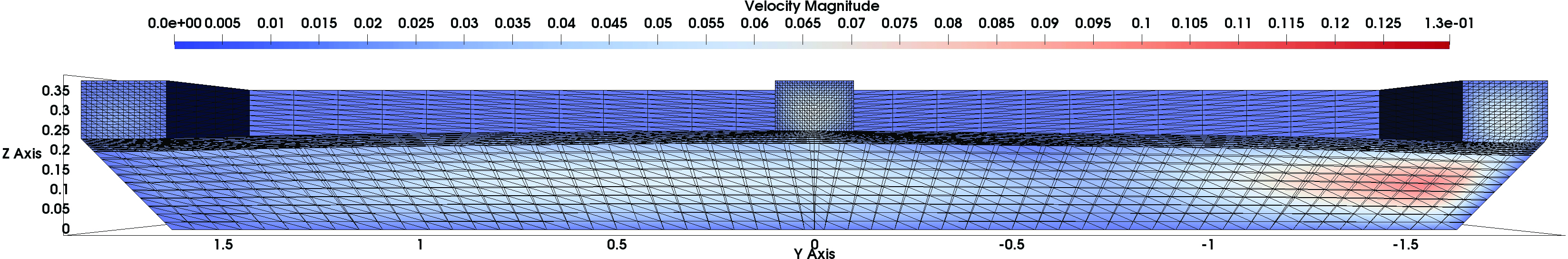
Reference industrial mesh (326099 vertices) and solution after solving the free-surface problem.

Adapted mesh (24255 vertices) and solution after solving the free-surface problem.
Cut at

Reference industrial mesh (326099 vertices) and solution after solving the free-surface problem.

Adapted mesh (24255 vertices) and solution after solving the free-surface problem.

Plot along y at

Plot along z at
8 Conclusion and Perspectives
An anisotropic error estimator for the approximation of a p-Laplacian problem is introduced. The constants involved in the upper and lower bounds are shown to be independent from the aspect ratio, the solution and μ, up to higher order terms. An adaptive algorithm based on the derived error estimator (4.12) is presented. Numerical experiments for
Funding statement: Paride Passelli is financed by Rio Tinto Aluminium LRF Research Center at Saint Jean de Maurienne (EPFL industrial grant).
Acknowledgements
Alexei Lozinski is acknowledged for advice. Maude Girardin, Samuel Dubuis and Jacques Rappaz are acknowledged for discussions. The referees are acknowledged for fruitful suggestions.
References
[1] M. Ainsworth and J. T. Oden, A posteriori error estimation in finite element analysis, Comput. Methods Appl. Mech. Engrg. 142 (1997), no. 1–2, 1–88. 10.1016/S0045-7825(96)01107-3Search in Google Scholar
[2] M. Ainsworth, J. Z. Zhu, A. W. Craig and O. C. Zienkiewicz, Analysis of the Zienkiewicz–Zhu a posteriori error estimator in the finite element method, Internat. J. Numer. Methods Engrg. 28 (1989), no. 9, 2161–2174. 10.1002/nme.1620280912Search in Google Scholar
[3] F. Alauzet and A. Loseille, A decade of progress on anisotropic mesh adaptation for computational fluid dynamics, Comput.-Aided Des. 72 (2016), 13–39. 10.1016/j.cad.2015.09.005Search in Google Scholar
[4] I. Babuška, J. Chandra and J. E. Flaherty, Adaptive Computational Methods for Partial Differential Equations, Society for Industrial and Applied Mathematics, Philadelphia, 1983. Search in Google Scholar
[5] I. Babuška, R. Durán and R. Rodríguez, Analysis of the efficiency of an a posteriori error estimator for linear triangular finite elements, SIAM J. Numer. Anal. 29 (1992), no. 4, 947–964. 10.1137/0729058Search in Google Scholar
[6] E. Bänsch, Local mesh refinement in 2 and 3 dimensions, Impact Comput. Sci. Engrg. 3 (1991), no. 3, 181–191. 10.1016/0899-8248(91)90006-GSearch in Google Scholar
[7] J. W. Barrett and W. B. Liu, Quasi-norm error bounds for the finite element approximation of a non-Newtonian flow, Numer. Math. 68 (1994), no. 4, 437–456. 10.1007/s002110050071Search in Google Scholar
[8] L. Belenki, L. Diening and C. Kreuzer, Optimality of an adaptive finite element method for the p-Laplacian equation, IMA J. Numer. Anal. 32 (2012), no. 2, 484–510. 10.1093/imanum/drr016Search in Google Scholar
[9] E. Boey, Y. Bourgault and T. Giordano, Anisotropic space-time adaptation for reaction-diffusion problems, preprint (2017), https://arxiv.org/abs/1707.04787. Search in Google Scholar
[10] Y. Bourgault and M. Picasso, Anisotropic error estimates and space adaptivity for a semidiscrete finite element approximation of the transient transport equation, SIAM J. Sci. Comput. 35 (2013), no. 2, A1192–A1211. 10.1137/120891320Search in Google Scholar
[11] W. Cao, Superconvergence analysis of the linear finite element method and a gradient recovery postprocessing on anisotropic meshes, Math. Comp. 84 (2015), no. 291, 89–117. 10.1090/S0025-5718-2014-02846-9Search in Google Scholar
[12] C. Carstensen, All first-order averaging techniques for a posteriori finite element error control on unstructured grids are efficient and reliable, Math. Comp. 73 (2004), no. 247, 1153–1165. 10.1090/S0025-5718-03-01580-1Search in Google Scholar
[13] C. Carstensen and R. Klose, A posteriori finite element error control for the p-Laplace problem, SIAM J. Sci. Comput. 25 (2003), no. 3, 792–814. 10.1137/S1064827502416617Search in Google Scholar
[14] C. Carstensen, W. Liu and N. Yan, A posteriori FE error control for p-Laplacian by gradient recovery in quasi-norm, Math. Comp. 75 (2006), no. 256, 1599–1616. 10.1090/S0025-5718-06-01819-9Search in Google Scholar
[15] P. Clément, Approximation by finite element functions using local regularization, Rev. Franç. Automat. Inform. Rech. Opér. Sér. Rouge Anal. Numér. 9 (1975), no. R-2, 77–84. 10.1051/m2an/197509R200771Search in Google Scholar
[16] T. Coupez, Metric construction by length distribution tensor and edge based error for anisotropic adaptive meshing, J. Comput. Phys. 230 (2011), no. 7, 2391–2405. 10.1016/j.jcp.2010.11.041Search in Google Scholar
[17] L. Diening and C. Kreuzer, Linear convergence of an adaptive finite element method for the p-Laplacian equation, SIAM J. Numer. Anal. 46 (2008), no. 2, 614–638. 10.1137/070681508Search in Google Scholar
[18] W. Dörfler, A convergent adaptive algorithm for Poisson’s equation, SIAM J. Numer. Anal. 33 (1996), no. 3, 1106–1124. 10.1137/0733054Search in Google Scholar
[19] S. Dubuis, Adaptive algorithms for two fluids flows with anisotropic finite elements and order two time discretizations, Ph.D. Thesis, Ecole polytechnique fédérale de Lausanne, 2019. Search in Google Scholar
[20] S. Dubuis, P. Passelli and M. Picasso, Anisotropic adaptive finite elements for an elliptic problem with strongly varying diffusion coefficient, Comput. Methods Appl. Math. 22 (2022), no. 3, 529–543. 10.1515/cmam-2022-0036Search in Google Scholar
[21] L. Formaggia, S. Micheletti and S. Perotto, Anisotropic mesh adaption in computational fluid dynamics: Application to the advection-diffusion-reaction and the Stokes problems, Appl. Numer. Math. 51 (2004), no. 4, 511–533. 10.1016/j.apnum.2004.06.007Search in Google Scholar
[22] L. Formaggia and S. Perotto, New anisotropic a priori error estimates, Numer. Math. 89 (2001), no. 4, 641–667. 10.1007/s002110100273Search in Google Scholar
[23] L. Formaggia and S. Perotto, Anisotropic error estimates for elliptic problems, Numer. Math. 94 (2003), no. 1, 67–92. 10.1007/s00211-002-0415-zSearch in Google Scholar
[24] P. J. Frey and F. Alauzet, Anisotropic mesh adaptation for CFD computations, Comput. Methods Appl. Mech. Engrg. 194 (2005), no. 48–49, 5068–5082. 10.1016/j.cma.2004.11.025Search in Google Scholar
[25] R. Glowinski and A. Marrocco, Sur l’approximation, par éléments finis d’ordre un, et la résolution, par pénalisation-dualité, d’une classe de problèmes de Dirichlet non linéaires, Rev. Franç. Automat. Inform. Rech. Opér. Sér. Rouge Anal. Numér. 9 (1975), no. R-2, 41–76. 10.1051/m2an/197509R200411Search in Google Scholar
[26] O. Gorynina, A. Lozinski and M. Picasso, Time and space adaptivity of the wave equation discretized in time by a second-order scheme, IMA J. Numer. Anal. 39 (2019), no. 4, 1672–1705. 10.1093/imanum/dry048Search in Google Scholar
[27] G. Kunert, An a posteriori residual error estimator for the finite element method on anisotropic tetrahedral meshes, Numer. Math. 86 (2000), no. 3, 471–490. 10.1007/s002110000170Search in Google Scholar
[28] G. Kunert and S. Nicaise, Zienkiewicz–Zhu error estimators on anisotropic tetrahedral and triangular finite element meshes, M2AN Math. Model. Numer. Anal. 37 (2003), no. 6, 1013–1043. 10.1051/m2an:2003065Search in Google Scholar
[29] G. Kunert and R. Verfürth, Edge residuals dominate a posteriori error estimates for linear finite element methods on anisotropic triangular and tetrahedral meshes, Numer. Math. 86 (2000), no. 2, 283–303. 10.1007/PL00005407Search in Google Scholar
[30] P. Laug and H. Borouchaki, The BL2D mesh generator – Beginner’s guide, user’s and programmer’s manual, Technical Report RT-0194, Institut National de Recherche en Informatique et Automatique (INRIA), Rocquencourt-Le Chesnay, 1996. Search in Google Scholar
[31] J.-L. Lions, Optimal Control of Systems Governed by Partial Differential Equations, Grundlehren Math. Wiss. 170, Springer, New York, 1971. 10.1007/978-3-642-65024-6Search in Google Scholar
[32] W. Liu and N. Yan, Quasi-norm local error estimators for p-Laplacian, SIAM J. Numer. Anal. 39 (2001), no. 1, 100–127. 10.1137/S0036142999351613Search in Google Scholar
[33] W. Liu and N. Yan, Some a posteriori error estimators for p-Laplacian based on residual estimation or gradient recovery, J. Sci. Comput. 16 (2001), no. 4, 435–477. Search in Google Scholar
[34] W. B. Liu and J. W. Barrett, Quasi-norm error bounds for the finite element approximation of some degenerate quasilinear elliptic equations and variational inequalities, RAIRO Modél. Math. Anal. Numér. 28 (1994), no. 6, 725–744. 10.1051/m2an/1994280607251Search in Google Scholar
[35] A. Loseille and F. Alauzet, Continuous mesh framework part I: Well-posed continuous interpolation error, SIAM J. Numer. Anal. 49 (2011), no. 1, 38–60. 10.1137/090754078Search in Google Scholar
[36] A. Lozinski, M. Picasso and V. Prachittham, An anisotropic error estimator for the Crank–Nicolson method: Application to a parabolic problem, SIAM J. Sci. Comput. 31 (2009), no. 4, 2757–2783. 10.1137/080715135Search in Google Scholar
[37] S. Micheletti and S. Perotto, Reliability and efficiency of an anisotropic Zienkiewicz–Zhu error estimator, Comput. Methods Appl. Mech. Engrg. 195 (2006), no. 9–12, 799–835. 10.1016/j.cma.2005.02.009Search in Google Scholar
[38] S. Micheletti, S. Perotto and M. Picasso, Stabilized finite elements on anisotropic meshes: A priori error estimates for the advection-diffusion and the Stokes problems, SIAM J. Numer. Anal. 41 (2003), no. 3, 1131–1162. 10.1137/S0036142902403759Search in Google Scholar
[39]
J.-M. Mirebeau,
Optimally adapted meshes for finite elements of arbitrary order and
[40] M. Picasso, Adaptive finite elements for a linear parabolic problem, Comput. Methods Appl. Mech. Engrg. 167 (1998), no. 3–4, 223–237. 10.1016/S0045-7825(98)00121-2Search in Google Scholar
[41] M. Picasso, An anisotropic error indicator based on Zienkiewicz–Zhu error estimator: Application to elliptic and parabolic problems, SIAM J. Sci. Comput. 24 (2003), no. 4, 1328–1355. 10.1137/S1064827501398578Search in Google Scholar
[42] M. Picasso, Numerical study of the effectivity index for an anisotropic error indicator based on Zienkiewicz–Zhu error estimator, Comm. Numer. Methods Engrg. 19 (2003), no. 1, 13–23. 10.1002/cnm.546Search in Google Scholar
[43] M. Picasso, Adaptive finite elements with large aspect ratio based on an anisotropic error estimator involving first order derivatives, Comput. Methods Appl. Mech. Engrg. 196 (2006), no. 1–3, 14–23. 10.1016/j.cma.2005.11.018Search in Google Scholar
[44]
M. Picasso,
Numerical study of an anisotropic error estimator in the
[45] S. B. Pope, Turbulent flows, Meas. Sci. Technol 12 (2001), Paper No. 11. 10.1088/0957-0233/12/11/705Search in Google Scholar
[46] J. Rochat, Approximation numérique des coulements turbulents dans des cuves d’électrolyse de l’aluminium, Ph.D. Thesis, Ecole polytechnique fédérale de Lausanne, 2016. Search in Google Scholar
[47] R. Verfürth, A posteriori error estimation and adaptive mesh-refinement techniques, J. Comput. Appl. Math. 50 (1994), no. 1–3, 67–83. 10.1016/0377-0427(94)90290-9Search in Google Scholar
[48] R. Verfürth, A Review of A Posteriori Error Estimation and Adaptive Mesh-Refinement Techniques, Wiley-Teubner, New York, 1996. Search in Google Scholar
[49] R. Verfürth, A Posteriori Error Estimation Techniques for Finite Element Methods, Oxford University, Oxford, 2013. 10.1093/acprof:oso/9780199679423.001.0001Search in Google Scholar
[50] J. Xu and Z. Zhang, Analysis of recovery type a posteriori error estimators for mildly structured grids, Math. Comp. 73 (2004), no. 247, 1139–1152. 10.1090/S0025-5718-03-01600-4Search in Google Scholar
[51] O. C. Zienkiewicz and J. Z. Zhu, A simple error estimator and adaptive procedure for practical engineering analysis, Internat. J. Numer. Methods Engrg. 24 (1987), no. 2, 337–357. 10.1002/nme.1620240206Search in Google Scholar
[52] O. C. Zienkiewicz and J. Z. Zhu, The superconvergent patch recovery and a posteriori error estimates. I. The recovery technique, Internat. J. Numer. Methods Engrg. 33 (1992), no. 7, 1331–1364. 10.1002/nme.1620330702Search in Google Scholar
[53] Spatial Corp Headquarters, Broomfield, 3D Precise Mesh, https://www.3ds.com/. Search in Google Scholar
© 2024 Walter de Gruyter GmbH, Berlin/Boston
This work is licensed under the Creative Commons Attribution 4.0 International License.
Articles in the same Issue
- Frontmatter
- In Memoriam of Raytcho Lazarov
- A Finite Element Analysis in Balanced Norms for a Coupled System of Singularly Perturbed Reaction-Diffusion Equations
- Analysis of a Combined Spherical Harmonics and Discontinuous Galerkin Discretization for the Boltzmann Transport Equation
- On Error Estimates of a Discontinuous Galerkin Method of the Boussinesq System of Equations
- Finite Element Formulations for Maxwell’s Eigenvalue Problem Using Continuous Lagrangian Interpolations
- Variational Approximation for a Non-Isothermal Coupled Phase-Field System: Structure-Preservation & Nonlinear Stability
- Error Analysis of the Vector Penalty-Projection Methods for the Time-Dependent Stokes Equations with Open Boundary Conditions
- Numerical Analysis of a Second-Order Algorithm for the Time-Dependent Natural Convection Problem
- A Space-Time Finite Element Method for the Eddy Current Approximation of Rotating Electric Machines
- A P 2 H-Div-Nonconforming-H-Curl Finite Element for the Stokes Equations on Triangular Meshes
- An Inverse Matrix Eigenvalue Problem for Constructing a Vibrating Rod
- Anisotropic Adaptive Finite Elements for a p-Laplacian Problem
- On an Optimal AFEM for Elastoplasticity