Nonlinear analysis of generalized thermoelastic interaction in unbounded thermoelastic media
-
Zuhur Alqahtani
 ,
Alaa A. El-Bary
,
Alaa A. El-Bary

Abstract
The transient response of thermoelastic materials subjected to a time-decaying thermal field is presented in this article using a nonlinear analysis. The basic equations provided are based on a generalized thermoelastic model under changing thermal conductivity, which is incorporated into the formulations. This problem is solved using the finite-element techniques instead of the Kirchhoff transforms since solving non-linear equations is quite difficult. Laplace transformation and the eigenvalue approaches are used to solve the problems in the linear context of the Kirchhoff transforms. The study investigates and compares the impact of varying thermal conductivity both with and without employing Kirchhoff’s transform. The numerical outputs are graphically shown to display the displacement, temperature, and stress variations.
Nomenclature
-
-
Displacement components
-
-
Decayed heat flux exponent
-
-
Medium temperature
-
-
Non-positive parameter
-
-
Thermal relaxation time
-
-
Components of the stress
-
-
Kronecker symbol
-
-
Thermal conductivity when
-
-
Specific heat
-
-
Lame’s constants
-
-
Initial temperature of the medium
-
-
Linear thermal expansion coefficient
-
-
Mass density of tissue
-
-
Strain components
-
-
Tissue thermal conductivity
-
-
time
1 Introduction
Earlier perspectives presumed the independence of all thermal parameters in thermoelasticity models from temperature fluctuations. However, a more nuanced understanding emerged as Noda [1] extensively analyzed materials in 1991, demonstrating that thermal conductivity exponentially decreases with increasing temperature. The importance of thermoelastic material with varying thermal conductivity has increased, finding recent applications in intriguing fields, particularly in cutting-edge technology, notably within emerging energy sources.
In the thermoelastic field, employing the classical elastic model for heating conduction is well-suited for a wide range of engineering applications. Nevertheless, in scenarios involving ultrafast heating, the classical model falls short in providing precise temperature approximations. Generalized thermoelastic theory, which characterizes the interaction between mechanical and thermal loads in materials, introduces thermoelastic disturbances that propagate as waves with speeds more closely reflecting real-world behavior compared to the classical model proposed by Biot [2]. Consequently, to address these limitations and enhance the accuracy of temperature distribution determinations, various non-classical thermoelastic theories, including the Lord and Shulman (LS) [3] and Green and Naghdi [4,5] models, have been introduced.
As temperatures rise, it is conceivable that the properties of the materials may experience a reduction. In numerous materials, the thermal conductivity (K) typically reduces nearly linearly with rising absolute temperature (T) [6]. To solve the problem associated with varying thermal conductivity [7], Kirchhoff’s transformation mapping technique [6] is applied. For a one-dimensional problem involving varying material parameters, Mukhopadhyay and Kumar [8] employed the finite differences method.
Sherief and Hamza [9] proposed a model to account for the change in thermal conductivity in thermoelastic cylinders extending to infinity. Abbas et al. [10] investigated the interactions between light and heat within a semiconductor material featuring a cylindrical hole and changed thermal conductivity. Othman et al. [11] investigated the impacts of initial stress and varying thermal conductivity in infinite fibre-reinforced plates. Ghasemi et al. [12] studied the thermal analysis studying on convective fins with changes in thermal conductivity and heating generation. Xiong et al. [13] discussed analyzing the impacts of change thermal conduction in thermoelastic interactions within an anisotropic fiber-reinforced medium. Khoukhi et al. [14] examined the influence of changing thermal conductivity on transient temperature fluctuation within wall-embedded insulations. Abbas [15] utilized a finite-element approach to study magneto-thermoelasticity interactions in inhomogeneous isotropic cylinders. Xiong and Guo [16] investigated the impact of movable heat sources and varying properties in the context of magneto-thermoelastic, employing a fractional thermoelasticity theory. Zenkour and Abbas [17] examined a scenario that included density and thermoelastic properties varying with temperature, revealing important characteristics of materials exhibiting such temperature-dependent properties. Othman [18] investigated thermoelastic interaction in a two-dimensional thermoelasticity problem with temperature-dependence elastic modulus. Aboueregal and Sedighi [19] applied the Moore–Gibson–Thompson theory to examine the influences of rotations and evolving properties in visco-thermoelasticity anisotropic cylinders. The model considers the impacts of rotations and evolving properties, which can have a significant effect on heat transfer. Youssef and Abbas [20] conducted research on an unbounded medium containing spherical cavities, exploring how the heat conductive and elastic modulus change with temperature in materials. Several experimental and theoretical inquiries have consistently demonstrated a substantial association between temperature variations and thermal conductivity. Proposed solutions for a variety of issues have been derived through the utilization of extended thermoelastic models [21,22,23,24,25,26,27,28,29,30,31,32,33,34,35,36,37,38,39,40].
In this work, the effects of changes in relaxation time and thermal conductivity on the propagation of thermoelastic waves in different materials are going to be investigated. The nonlinear problems were solved by the finite-element methods (FEMs) without the necessity for the Kirchhoff transformation. Using eigenvalue analysis and Laplace transforms, solutions were found for the linear problems that included Kirchhoff’s transformations. The numerical results for various physical parameters were acquired and shown graphically. Through a close examination of the solution’s behavior, this study sought to confirm the accuracy and reliability of the proposed approach.
2 Basic equations
Consider elastic materials with constant elastic parameters, adhering to the fundamental relations within the framework of the generalized thermoelastic model. This model, which involves one relaxation time and assumes a linear variation of thermal conductivity within a specified temperature range, is utilized. Notably, nobody forces or heat source is considered, leading to the basic formulations that can be written by [3]
In this case,
Study an elastic material whose conditions are given as a function of both time (
3 Application
To derive solutions for the formulations, the initial and boundary conditions can be given by
To streamline the basic equations, we can employ the following dimensionless variables:
where
In relation to the dimensionless quantities defined in Eq. (10), the basic equations above are simplified (omitting the dashed notation for convenience):
where
3.1 Nonlinear model (FEM)
In this part, the basic equations were developed as nonlinear partial differential equations. FEMs are applied in this context to obtain solutions for Eqs. (11) and (12). The FEM, initially developed for the numerical solutions of intricate problems in structural mechanics, remains a preferred approach for complex systems. The standard processes of weak formulations, as outlined in [42,43], are utilized in these approaches. The weak non-dimensional formulation has been established through derivation from the fundamental relations. The explicit definitions of the sets of independent test functions, indicated by temperature
Here,
Subsequently, the time derivatives of the unidentified factors are computed by an implicit procedure. The weak formulations corresponding to the governing Eqs. (11) and (12) are presented below for the FEM analysis:
3.2 Linear model (Kirchhoff’s transform)
Now, to obtain the linearized forms of the governing equations from their original nonlinear state, Kirchhoff’s transformation mapping [41] is applied to account for the variation in thermal conductivity, as defined in Eq. (4)
This expression defines a new function that represents heat conduction. The integration is carried out after substituting the expressions from (19) in (4), yielding the result specified in Youssef [41]
In linear form, the governing Eqs. (11)–(14) can be expressed as
Utilizing Laplace transform on Eqs. (22)–(26),
Hence
The vector-matrix differential equations can be rewritten using the combined equations presented in (28) and (29)
where
By employing the eigenvalue techniques, as outlined in previous works [44,45,46,47,48,49,50,51,52], the characteristic formulation of matrix A can be given by
The matrix eigenvalue is characterized by the four roots of the formulation, expressed as
In this equation,
4 Results
Now, let us consider a numerical example to demonstrate the issue, utilizing an elastic isotropic material as the chosen material for numerical evaluations. The relevant physical data are provided as [15]
We studied how temperature, displacement, and stress change over distance in a material. We used a generalized thermoelastic model that includes one thermal relaxation time for heat transfer. Numerical simulations were run to model these physical properties. The simulations considered how thermal conductivity and other factors affect the results. Some simulations included Kirchhoff transforms, and some did not. Standard values were used for the initial temperature, displacement, and stress variations. The calculations were done at a time of

The effects of relaxation time in temperature variation via the distance.
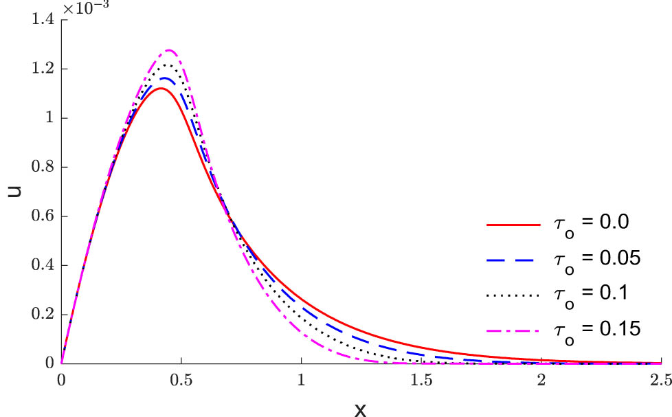
The effects of relaxation time in displacement variation via the distance.

The impacts of relaxation time on stress variation via the distance.
The effects of the exponent of decayed heating flux on the distributions of temperature via the distance.
The effects of the exponent of decayed heating flux on the distributions of displacement via the distance.
The effects of the exponent of decayed heating flux on the distributions of stress via the distance.
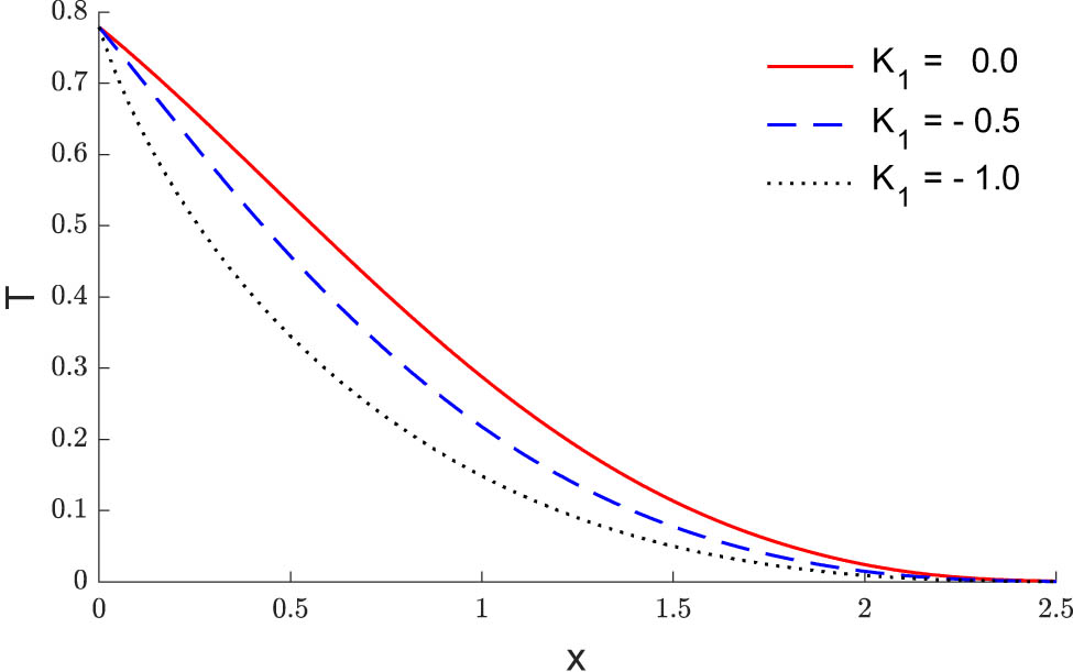
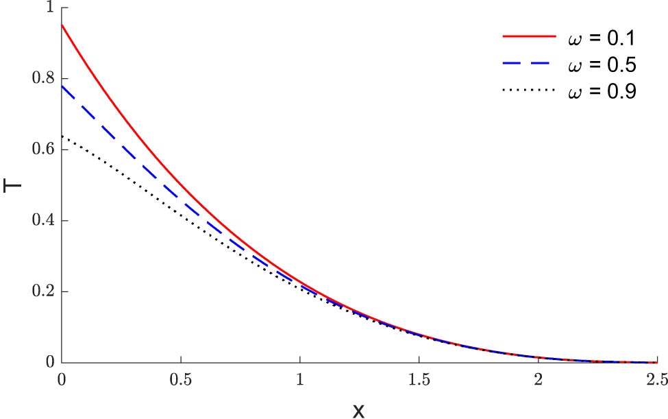
The temperature variations during the distances under varying thermal conductivity.
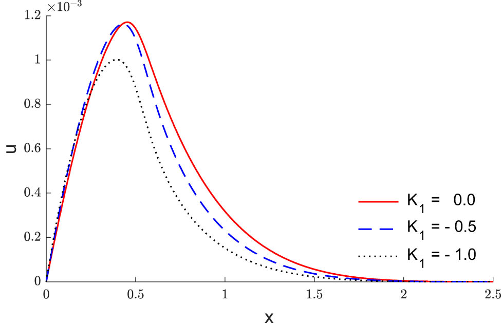
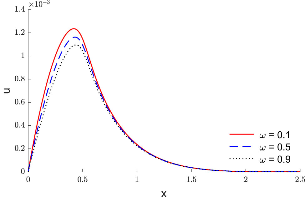
The displacement variation via the distances under varying thermal conductivity.
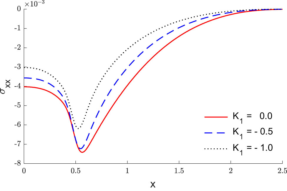
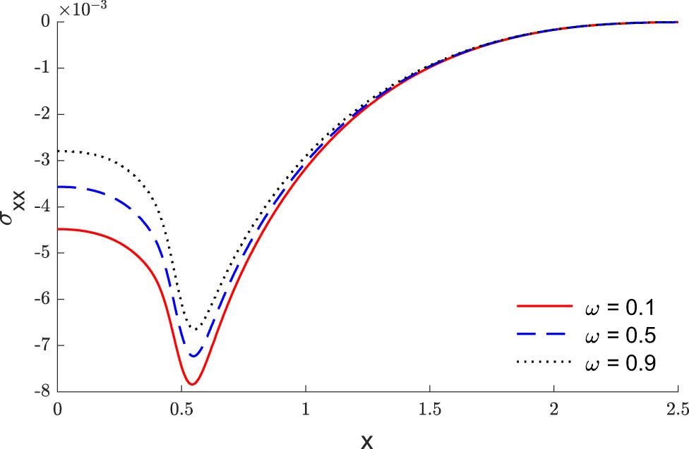
The stress variation via the distances under varying thermal conductivity.
The temperature change at

The displacement variations at

The stress variation at
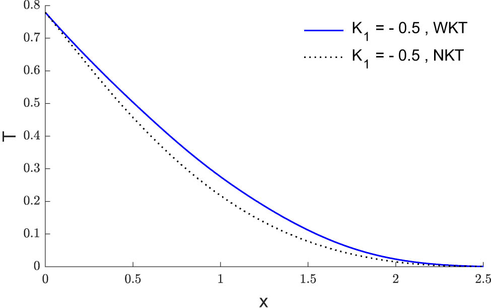
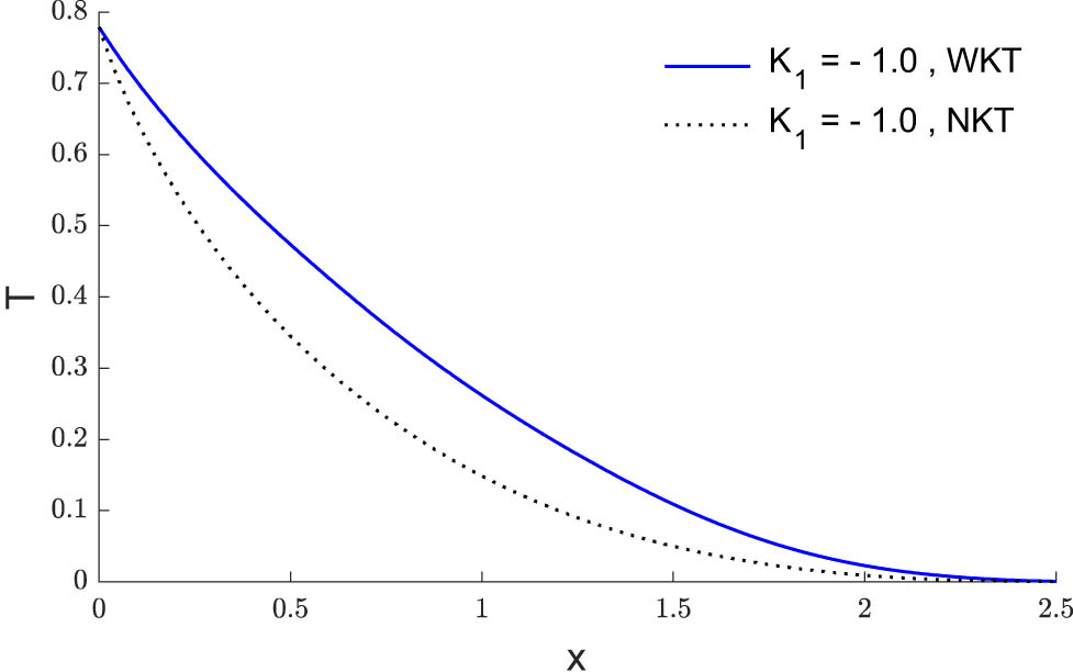
The temperature variation with and without the application of Kirchhoff’s transform, considering the thermal conductivity parameter

The displacement variation with and without the application of Kirchhoff’s transform, considering the thermal conductivity parameter
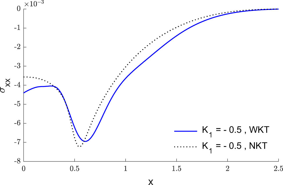
The stress variation with and without the application of Kirchhoff’s transforms, considering the thermal conductivity parameter

A comparison of changes in temperature when

A comparison of changes in displacement when

A comparison of changes in stress when
Figures 1, 4, 7, 10, 13, and 16 illustrate the temperature variations across distance
Figures 1–3 show a comparison of the outcomes obtained for physical parameters such as displacement, temperature, and stress, considering two models of thermoelasticity: the coupled theory without thermal relaxation time (
The impacts of the exponent of the decayed heating flux
Without using the Kirchhoff transforms, Figures 7–9 show the effects of variable thermal conductivity on the studying variables via distance
Figures 10–15 show a comparison of the results obtained when utilizing the Kirchhoff transform (WKT cases) versus not utilizing it (NKT cases). Specifically, these figures show the temperature variation, the displacement variation, and stress distribution via the distances
Figures 16–18 show a comparison of the analytical solution obtained using the Laplace transform and the eigenvalue approaches with Kirchhoff transforms versus the numerical solution from the FEMs without using Kirchhoff transforms. This comparison is shown for the case where
5 Conclusion
The transient thermoelastic response of materials under a time-decaying thermal field is examined in this work by employing nonlinear analysis techniques. The studying variable distributions were thoroughly understood by integrating varying thermal conductivity into a generalized thermoelasticity model with one thermal relaxation time. In solving nonlinear thermoelastic problems with variable thermal conductivity, the results demonstrate the robustness of the finite-element technique. This research study helps to comprehend the interactions existing between mechanical and thermal fields of a thermoelastic material which will further assist in better modeling in real applications.
Acknowledgments
This work was supported by the Princess Nourah bint Abdulrahman University Researchers Supporting Project number (PNURSP2025R518) and Princess Nourah bint Abdulrahman University, Riyadh, Saudi Arabia.
-
Funding information: This work was supported by the Princess Nourah bint Abdulrahman University Researchers Supporting Project number (PNURSP2025R518), and Princess Nourah bint Abdulrahman University, Riyadh, Saudi Arabia.
-
Author contributions: All authors have accepted responsibility for the entire content of this manuscript and consented to its submission to the journal, reviewed all the results and approved the final version of the manuscript. Conceptualization, Z.A., I.A., and A.A.; methodology, Z.A., I.A., and A.E.; software, Z.A., I.A., and A.E.; validation, I.A., A.E., and A.A.; formal analysis, I.A., A.E., and A.A.; investigation, Z.A., I.A., A.E., and A.A.; resources, A.A. All authors have read and agreed to publish version of the manuscript.
-
Conflict of interest: Authors state no conflict of interest.
References
[1] Noda N. Thermal stresses in materials with temperature-dependent properties. Appl Mech Rev. 1991;44(9):383–97.10.1115/1.3119511Suche in Google Scholar
[2] Biot MA. Thermoelasticity and irreversible thermodynamics. J Appl Phys. 1956;27(3):240–53.10.1063/1.1722351Suche in Google Scholar
[3] Lord HW, Shulman Y. A generalized dynamical theory of thermoelasticity. J Mech Phys Solids. 1967;15(5):299–309.10.1016/0022-5096(67)90024-5Suche in Google Scholar
[4] Green AE, Naghdi PM. Thermoelasticity without energy dissipation. J Elast. 1993;31(3):189–208.10.1007/BF00044969Suche in Google Scholar
[5] Green A, Naghdi P. A re-examination of the basic postulates of thermomechanics. Proc R Soc Lond Ser A: Math Phys Sci. 1991;432(1885):171–94.10.1098/rspa.1991.0012Suche in Google Scholar
[6] Hetnarski RB. Thermal stresses IV. North Holland: Elsevier; 1996.10.1080/01495739608946163Suche in Google Scholar
[7] Sherief H, Abd El-Latief AM. Effect of variable thermal conductivity on a half-space under the fractional order theory of thermoelasticity. Int J Mech Sci. 2013;74:185–9.10.1016/j.ijmecsci.2013.05.016Suche in Google Scholar
[8] Mukhopadhyay S, Kumar R. Solution of a problem of generalized thermoelasticity of an annular cylinder with variable material properties by finite difference method. Comput Methods Sci Technol. 2009;15(2):169–76.10.12921/cmst.2009.15.02.169-176Suche in Google Scholar
[9] Sherief HH, Hamza FA. Modeling of variable thermal conductivity in a generalized thermoelastic infinitely long hollow cylinder. Meccanica. 2015;51(3):551–8.10.1007/s11012-015-0219-8Suche in Google Scholar
[10] Abbas I, Hobiny A, Marin M. Photo-thermal interactions in a semi-conductor material with cylindrical cavities and variable thermal conductivity. J Taibah Univ Sci. 2020;14(1):1369–76.10.1080/16583655.2020.1824465Suche in Google Scholar
[11] Othman MIA, Abouelregal AE, Said SM. The effect of variable thermal conductivity on an infinite fiber-reinforced thick plate under initial stress. J Mech Mater Struct. 2019;14(2):277–93.10.2140/jomms.2019.14.277Suche in Google Scholar
[12] Ghasemi SE, Hatami M, Ganji DD. Thermal analysis of convective fin with temperature-dependent thermal conductivity and heat generation. Case Stud Therm Eng. 2014;4:1–8.10.1016/j.csite.2014.05.002Suche in Google Scholar
[13] Xiong CB, Yu LN, Niu YB. Effect of variable thermal conductivity on the generalized thermoelasticity problems in a fiber-reinforced anisotropic half-space. Adv Mater Sci Eng. 2019;2019:1–9.10.1155/2019/8625371Suche in Google Scholar
[14] Khoukhi M, Abdelbaqi S, Hassan A. Transient temperature change within a wall embedded insulation with variable thermal conductivity. Case Stud Therm Eng. 2020;20:100645.10.1016/j.csite.2020.100645Suche in Google Scholar
[15] Abbas IA. Generalized magneto-thermoelasticity in a nonhomogeneous isotropic hollow cylinder using the finite element method. Arch Appl Mech. 2009;79(1):41–50.10.1007/s00419-008-0206-9Suche in Google Scholar
[16] Xiong CB, Guo Y. Effect of variable properties and moving heat source on magnetothermoelastic problem under fractional order thermoelasticity. Adv Mater Sci Eng. 2016;2016:1–12.10.1155/2016/5341569Suche in Google Scholar
[17] Zenkour AM, Abbas IA. A generalized thermoelasticity problem of an annular cylinder with temperature-dependent density and material properties. Int J Mech Sci. 2014;84:54–60.10.1016/j.ijmecsci.2014.03.016Suche in Google Scholar
[18] Othman MI. Lord-Shulman theory under the dependence of the modulus of elasticity on the reference temperature in two-dimensional generalized thermoelasticity. J Therm Stresses. 2002;25(11):1027–45.10.1080/01495730290074621Suche in Google Scholar
[19] Aboueregal AE, Sedighi HM. The effect of variable properties and rotation in a visco-thermoelastic orthotropic annular cylinder under the Moore-Gibson-Thompson heat conduction model. Proc Inst Mech Eng Part L-J Mater-Des Appl. 2021;235(5):1004–20.10.1177/1464420720985899Suche in Google Scholar
[20] Youssef HM, Abbas IA. Thermal shock problem of generalized thermoelasticity for an infinitely long annular cylinder with variable thermal conductivity. Comput Methods Sci Technol. 2007;13(2):95–100.10.12921/cmst.2007.13.02.95-100Suche in Google Scholar
[21] Singh S, Kumar D, Rai KN. Convective-radiative fin with temperature dependent thermal conductivity, heat transfer coefficient and wavelength dependent surface emissivity. Propuls Power Res. 2014;3(4):207–21.10.1016/j.jppr.2014.11.003Suche in Google Scholar
[22] Zhang H, Shang C, Tang G. Measurement and identification of temperature-dependent thermal conductivity for thermal insulation materials under large temperature difference. Int J Therm Sci. 2022;171:107261.10.1016/j.ijthermalsci.2021.107261Suche in Google Scholar
[23] Pan W, Yi F, Zhu Y, Meng S. Identification of temperature-dependent thermal conductivity and experimental verification. Meas Sci Technol. 2016;27(7):075005.10.1088/0957-0233/27/7/075005Suche in Google Scholar
[24] Wang YZ, Zan C, Liu D, Zhou JZ. Generalized solution of the thermoelastic problem for the axisymmetric structure with temperature-dependent properties. Eur J Mech - A/Solids. 2019;76:346–54.10.1016/j.euromechsol.2019.05.004Suche in Google Scholar
[25] Wang YZ, Liu D, Wang Q, Zhou JZ. Thermoelastic interaction in functionally graded thick hollow cylinder with temperature-dependent properties. J Therm Stresses. 2018;41(4):399–417.10.1080/01495739.2017.1422823Suche in Google Scholar
[26] Wang Y, Liu D, Wang Q, Zhou J. Problem of axisymmetric plane strain of generalized thermoelastic materials with variable thermal properties. Eur J Mech - A/Solids. 2016;60:28–38.10.1016/j.euromechsol.2016.06.001Suche in Google Scholar
[27] Ezzat MA, El-Bary AA. On thermo-viscoelastic infinitely long hollow cylinder with variable thermal conductivity. Microsyst Technol. 2017;23(8):3263–70.10.1007/s00542-016-3101-2Suche in Google Scholar
[28] Hobiny A, Alzahrani F, Abbas I, Marin M. The effect of fractional time derivative of bioheat model in skin tissue induced to laser irradiation. Symmetry. 2020;12(4):1–10.10.3390/sym12040602Suche in Google Scholar
[29] Abbas IA. A GN model for thermoelastic interaction in an unbounded fiber-reinforced anisotropic medium with a circular hole. Appl Math Lett. 2013;26(2):232–9.10.1016/j.aml.2012.09.001Suche in Google Scholar
[30] Marin M, Florea O. On temporal behaviour of solutions in thermoelasticity of porous micropolar bodies. Analele Univ “Ovidius” Constanta - Ser Mat. 2014;22(1):169–88.10.2478/auom-2014-0014Suche in Google Scholar
[31] Bhatti MM, Marin M, Zeeshan A, Abdelsalam SI. Editorial: Recent trends in computational fluid dynamics. Front Phys. 2020;8:593111. 10.3389/fphy.2020.593111.Suche in Google Scholar
[32] Alzahrani FS, Abbas IA. Analytical estimations of temperature in a living tissue generated by laser irradiation using experimental data. J Therm Biol. 2019;85:102421.10.1016/j.jtherbio.2019.102421Suche in Google Scholar PubMed
[33] Hobiny A, Abbas I. Analytical solutions of fractional bioheat model in a spherical tissue. Mech Based Des Struct Mach. 2019;49(3):430–9.10.1080/15397734.2019.1702055Suche in Google Scholar
[34] Marin M, Seadawy A, Vlase S, Chirila A. On mixed problem in thermoelasticity of type III for Cosserat media. J Taibah Univ Sci. 2022;16(1):1264–74.10.1080/16583655.2022.2160290Suche in Google Scholar
[35] Othman MI, Fekry M, Marin M. Plane waves in generalized magneto-thermo-viscoelastic medium with voids under the effect of initial stress and laser pulse heating. Struct Eng Mech. 2020;73(6):621–9.Suche in Google Scholar
[36] Marin M. Some estimates on vibrations in thermoelasticity of dipolar bodies. J Vib Control. 2010;16(1):33–47.10.1177/1077546309103419Suche in Google Scholar
[37] Cong PH, Duc ND. Nonlinear thermo-mechanical analysis of ES double curved shallow auxetic honeycomb sandwich shells with temperature-dependent properties. Compos Struct. 2022;279:114739.10.1016/j.compstruct.2021.114739Suche in Google Scholar
[38] Shahmohammadi MA, Mirfatah SM, Emadi S, Salehipour H, Civalek Ö. Nonlinear thermo-mechanical static analysis of toroidal shells made of nanocomposite/fiber reinforced composite plies surrounded by elastic medium. Thin-Walled Struct. 2022;170:108616.10.1016/j.tws.2021.108616Suche in Google Scholar
[39] Tornabene F, Viscoti M, Dimitri R. Thermo-mechanical analysis of laminated doubly-curved shells: Higher order equivalent layer-wise formulation. Compos Struct. 2024;335:117995.10.1016/j.compstruct.2024.117995Suche in Google Scholar
[40] Farokhi H, Ghayesh MH. Nonlinear thermo-mechanical behaviour of MEMS resonators. Microsyst Technol. 2017;23:5303–15.10.1007/s00542-017-3381-1Suche in Google Scholar
[41] Youssef H. State-space approach on generalized thermoelasticity for an infinite material with a spherical cavity and variable thermal conductivity subjected to ramp-type heating. Can Appl Math Quaterly. 2005;13:4.Suche in Google Scholar
[42] Zenkour AM, Abbas IA. Nonlinear transient thermal stress analysis of temperature-dependent hollow cylinders using a finite element model. Int J Struct Stab Dyn. 2014;14(7):1450025.10.1142/S0219455414500254Suche in Google Scholar
[43] Abbas IA, Kumar R. 2D deformation in initially stressed thermoelastic half-space with voids. Steel Compos Struct. 2016;20(5):1103–17.10.12989/scs.2016.20.5.1103Suche in Google Scholar
[44] Abbas IA. Eigenvalue approach on fractional order theory of thermoelastic diffusion problem for an infinite elastic medium with a spherical cavity. Appl Math Model. 2015;39(20):6196–206.10.1016/j.apm.2015.01.065Suche in Google Scholar
[45] Abbas IA, Abdalla AENN, Alzahrani FS, Spagnuolo M. Wave propagation in a generalized thermoelastic plate using eigenvalue approach. J Therm Stresses. 2016;39(11):1367–77.10.1080/01495739.2016.1218229Suche in Google Scholar
[46] Othman MIA, Abbas IA. Eigenvalue approach for generalized thermoelastic porous medium under the effect of thermal loading due to a laser pulse in DPL model. Indian J Phys. 2019;93(12):1567–78.10.1007/s12648-019-01431-9Suche in Google Scholar
[47] Kumar R, Miglani A, Rani R. Eigenvalue formulation to micropolar porous thermoelastic circular plate using dual phase lag model. Multidiscipline Modeling in. Mater Struct. 2017;13(2):347–62.10.1108/MMMS-08-2016-0038Suche in Google Scholar
[48] Kumar R, Miglani A, Rani R. Analysis of micropolar porous thermoelastic circular plate by eigenvalue approach. Arch Mech. 2016;68(6):423–39.Suche in Google Scholar
[49] Gupta ND, Das NC. Eigenvalue approach to fractional order generalized thermoelasticity with line heat source in an infinite medium. J Therm Stresses. 2016;39(8):977–90.10.1080/01495739.2016.1187987Suche in Google Scholar
[50] Santra S, Lahiri A, Das NC. Eigenvalue approach on thermoelastic interactions in an infinite elastic solid with voids. J Therm Stresses. 2014;37(4):440–54.10.1080/01495739.2013.870854Suche in Google Scholar
[51] Baksi A, Roy BK, Bera RK. Eigenvalue approach to study the effect of rotation and relaxation time in generalized magneto-thermo-viscoelastic medium in one dimension. Math Comput Model. 2006;44(11–12):1069–79.10.1016/j.mcm.2006.03.010Suche in Google Scholar
[52] Das NC, Lahiri A, Giri RR. Eigenvalue approach to generalized thermoelasticity. Indian J Pure Appl Math. 1997;28(12):1573–94.Suche in Google Scholar
[53] Stehfest H. Algorithm 368: Numerical inversion of Laplace transforms [D5]. Commun ACM. 1970;13(1):47–9.10.1145/361953.361969Suche in Google Scholar
© 2025 the author(s), published by De Gruyter
This work is licensed under the Creative Commons Attribution 4.0 International License.
Artikel in diesem Heft
- Research Articles
- Layerwise generalized formulation solved via a boundary discontinuous method for multilayered structures. Part 1: Plates
- Thermoelastic interactions in functionally graded materials without energy dissipation
- Layerwise generalized formulation solved via boundary discontinuous method for multilayered structures. Part 2: Shells
- Visual scripting approach for structural safety assessment of masonry walls
- Nonlinear analysis of generalized thermoelastic interaction in unbounded thermoelastic media
- Study of heat transfer through functionally graded material fins using analytical and numerical investigations
- Analysis of magneto-aerothermal load effects on variable nonlocal dynamics of functionally graded nanobeams using Bernstein polynomials
- Effective thickness of gallium arsenide on the transverse electric and transverse magnetic modes
- Investigating the behavior of above-ground concrete tanks under the blast load regarding the fluid-structure interaction
- Numerical study on the effect of V-notch on the penetration of grounding incidents in stiffened plates
- Thermo-elastic analysis of curved beam made of functionally graded material with variable parameters
- Effect of curved geometrical aspects of Savonius rotor on turbine performance using factorial design analysis
- A mechanical and microstructural investigation of friction stir processed AZ31B Mg alloy-SiC composites
- Mechanical design of engineered-curved patrol boat hull based on the geometric parameters and hydrodynamic criteria
- Analysis of functionally graded porous plates using an enhanced MITC3+ element with in-plane strain correction
- Review Article
- Technological developments of amphibious aircraft designs: Research milestone and current achievement
- Special Issue: TS-IMSM 2024
- Influence of propeller shaft angles on the speed performance of composite fishing boats
- Design optimization of Bakelite support for LNG ISO tank 40 ft using finite element analysis