The Connections among the US, China and Russia through Safe Assets

2.1 Model Setup

There are three periods t=0°, t=0 and t=1 and a single good. The single good is understood as the composite of all commodities circulating in global economy. The endowment of this good by the US, China and Russia are w, w^* and w^** respectively.

The strategic interaction among the US, China and Russia in the model cover the following categories: the Nash bargaining between the Central Bank of China, i.e. People’s Bank of China, and the Ministry of Finance of China over the country’s endowment at t=0°; the safe asset transaction between the U.S. Treasury and People’s Bank of China at t=0; the safe asset transaction between the Finance Ministry of China and Bank of Russia at t=0; the trade-off between debt issuance and devaluing USD between the U.S. Treasury and the Federal Reserve.

Consider the safe asset transaction between the U.S. Treasury and People’s Bank of China. Beyond the safe asset transaction, at the mean time, both the U.S. Treasury and People’s Bank of China need some risky real assets to either satisfy their intertemporal consumption optimization purpose or portfolio optimization purpose respectively. The risky real asset happens to be there in the safe asset transaction between the U.S. Treasury and People’s Bank of China are named by, ’the first risky real asset’. The first risky real asset is in perfectly elastic supply and denoted by USD. The nominal bonds, denoted in USD, are issued by the U.S. Treasury to People’s Bank of China.

Within the above strategic interaction, the US encounters two states related to its macroeconomic environment at t=1, which are indexed by H and L. The L state represents a disaster in the macroeconomic environment of the US, which occurs with probability λ ∈ (0, 1). Instead, the H state represents a positive status of the macroeconomic environment of the US, which occurs with the remaining probability 1-λ. Farhi and Maggiori (2018) use the same specification to describe the state US may encounter, and this paper follows their style as well.

The exogenous real return of the first risky real asset is denoted by R^r. In state H, its return is RHr > 1; in state L, its return is RLr < 1. I use the notations R^r and σ² to represent the expected return and riskiness of the first risky real asset, i.e., Rr¯=ERr=(1−λ)RHr+λRLr and σ² = Var(R^r).

Both the Ministry of Finance of China and Bank of Russia are willing to invest in some risky asset to satisfy their intertemporal consumption optimization purpose and portfolio optimization purpose respectively. The risky real asset that happens to be there in the strategic interaction between Ministry of Finance of China and Central Bank of Russia is called the second risky real asset. The second risky real asset is in perfectly elastic supply and also denoted by USD. The nominal bonds, denoted in USD, are issued by the Ministry of Finance of China to Central Bank of Russia.

In the interaction between the Ministry of Finance of China and Bank of Russia, because the Chinese debt is also denoted by USD, therefore the Ministry of Finance of China is also specified to encounter the two states H and L which the US encounters. That means, when the US is in good state, then China is also in good state; when the US is in bad state, China is also in bad state. Whether the US devalues USD or not determines the value of Chinese debt. China is tied with the climate of the US macroeconomic environment due to the denomination of Chinese debt by USD.

The exogenous real return of the second risky real asset is denoted as R^r*. In state H, its return is RHr∗>1; in state L, its return is RLr∗<1. I use the notations R^r* and σ^*2 to denote the expected return and riskiness of the second risky real asset, i.e., Rr∗¯=ERr∗=1−λ∗RHr∗+λ∗RLr∗ and σ^*2 = Var(R^r*).

The following short-hand notations for expectation operators will be used to describe the model. It also helps understand the timing to the model. These expectation operators are referred from Farhi and Maggiori (2018), which also apply in this context. Keeping the consistency of notations helps understand the connection and differences between Farhi and Maggiori (2018) and my model:

Definition (Farhi and Maggiori (2018)): Define E⁺ [x₁] to denote the expectation taken at time t=0⁺ of random variable x₁ the realization of which will occur at t=1. Further define E^s [x₁] to be the expectation taken at t=0⁺ conditional on the safe realization of the sunspot, and E^r [x₁] to be the expectation taken at t=0⁺ conditional on the risky realization of the sunspot. Define E^- [ x₁] to be the expectation taken at t=0^- before the sunspot realization.

Timing. The event sequence of the model is constructed based on the Calvo timing (Calvo, 1988). At the beginning ( t = t0o ), the People’s Bank of China and the Ministry of Finance of China bargains over how to divide the endowment of the country. The event sequence of my model is exhibited in Figure 1.

Figure 1

Event Sequence of the Model

The game proceeds as follows. At t=0^o, People’s Bank of China and the Ministry of Finance of China bargains over the endowment of China to determine the share each entity possesses. At the meantime, the endowment of the US and Russia are also determined.

At t=0^-, the U.S. Treasury determines the amount of reserve asset that will be issued to People’s Bank of China; the Ministry of Finance of China determines the amount of reserve asset that will be issued to Russia. The Federal Reserve invests in the first real risky asset; People’s Bank of China invests in the first real risky asset and the Ministry of Finance of China invests in the second risky real asset; Bank of Russia invests in the second real risky asset. The U.S. Treasury and the Ministry of Finance of China determine their intertemporal consumption at t=0^-.

At t=0⁺, the interest rate about the amount of reserve asset determined by the US is determined by People’s Bank of China, which invests in the reserve asset; the interest rate about the amount of reserve asset issued by the Ministry of Finance of China is determined by Bank of Russia, which invests in the reserve asset. A sunspot for selecting equilibrium is realized for the safe asset transaction between the U.S. Treasury and People’s Bank of China; another sunspot for selecting equilibrium is realized for the safe asset transaction between the Ministry of China and Bank of Russia.

At t=1, supposing a disaster shock comes towards US, the Federal Reserve decides whether to devalue USD; the disaster shock that the US experiences also affects China due to the dollar-denomination of Chinese debt. People’s Bank of China will also consider whether or not to adjust the RMB value over RUB at t=1. However, People’s Bank of China will consider adjusting the value of RMB only if the US and China are off-equilibrium (Proposition 7). The consumption of the Federal Reserve and People’s Bank of China at period t=1 in their respective consumption optimization problems are determined. Besides, the consumption of Bank of Russia at period t=1 in their portfolio optimization problem is also determined.

At t=0^-, the U.S. Treasury needs determine the amount of the reserve asset to issue and its investment in the risky asset. I use b to denote the debt to issue at t=0^- and x to denote the first real risky asset to invest at t=0^-. By determining x and b, the consumption at t=0, C₀, is determined at t=0^-. The interest rate on the outstanding debt b is denoted by R. It is determined after t=0^-, which is the time point t=0⁺. At t=0⁺, the sunspot ω is realized. The sunspot has binary realizations: s indicates a safe equilibrium and it is realized with probability α; r indicates a risky equilibrium and it is realized with probability 1-α. Given the realization of the sunspot, an equilibrium is selected. The interest rate on the outstanding debt R is therefore determined given the realization of ω and b. Hence, the interest rate can be denoted by R(b, ω).

At t=1, if the macroeconomic environment of the US is positive, i.e., the state H happens, then no devaluations could happen; however, if the disaster state L happens, the US will consider whether to devalue USD, which is implemented by the Federal Reserve, to ease its burden to repay the debt or fulfill its commitment, which is conducted by the U.S. Treasury, by not devaluing USD. Therefore, I denote the exchange rate by e ∈ {1, e_L}, where e_L < 1. e represents the RMB price of a dollar. In state L, e=1 if the US fulfills its commitment to its debt and e < 1 if the US devalues USD to reduce the value of its debt. According to the event sequence, the choice of exchange rate is determined by the amount of the outstanding debt b and the potential sunspot ω. Therefore, the exchange rate at this time period can be denoted by e(b, ω).

Given the exchange rate, the consumption at period 1 expected before t=0⁺ can also be determined. I denote it by C₁(ω). The devaluation of USD is associated with the devaluation cost τ(1 – e (b, ω)). τ is a normalization constant and if USD is completely devalued, the devaluation cost is just ε.

Finally, because the U.S. Treasury meets an intertemporal consumption optimization problem, therefore I denote the discount factor by δ. To ensure the US is indifferent between the timing of consumption, I specify δ=1Rr¯. Note that C₀ and C₁(ω) are determined by the U.S. Treasury, while the Federal Reserve may adjust the value of USD contingently. The intertemporal consumption decision problem essentially reflects the trade-off between issuing more debt and keeping the value of USD by the U.S. Treasury and the Federal Reserve.

Based on all above ingredients, the intertemporal consumption problem of the US will be construetd. The U.S. Treasury and the Federal Reserve are assumed risk neutral over the consumption across the two periods. The payoff of the US is the total consumption of t=0 and t=1 minus the devaluation cost, which is given by:

The US needs to choose b, x, C₀ and C₁(ω) to maximize the above payoff. Given all above specification, the intertemporal consumption problem of the US is written by:

Next, this paper introduces the bargaining between People’s Bank of China and Ministry of Finance of China. In order to optimize its portfolio, People’s Bank of China invests b in the reserve asset issued by the US and x^* in the first real risky asset. It also needs to determine its consumption at t=1, which is denoted by C1∗ . People’s Bank of China has a mean-variance preference over consumption in which its risk aversion coefficient is denoted by γ. People’s Bank of China’s portfolio optimization problem is written in the following:

Note that in the above problem, w^*, x^*, b and C1∗ are denoted by USD. By solving the above portfolio optimization problem, People’s Bank of China determines its demand for the US debt. w^* has been determined at t=0^o.

At t=0^-, the Ministry of Finance of China needs to determine the amount of reserve asset to issue and its investment in the risky asset as well as its consumption at this period. I use b^* to denote the debt to issue at t=0^- and x∗^ to denote the amount of invested second real risky asset at t=0^-. By determining x∗^ and b^*, the consumption of the Ministry of Finance of China at t=0, C0∗ , is determined at t=0^-. The interest rate on the outstanding debt b^* is denoted by R^*. It is determined at t=0⁺. At t=0⁺, the sunspot ω^* is realized. The sunspot has binary realizations: s^* indicates a safe equilibrium and it is realized with probability α^*; r^* indicates a risky equilibrium and it is realized with probability 1-α^*. Given the realization of the sunspot, an equilibrium of the strategic interaction between the Ministry of Finance of China and Bank of Russia is selected. The interest rate on the outstanding debt is therefore determined given the realization of w^* and b^*. Hence, the interest rate R^* can be denoted by R^*(b^*, ω^*).

At t=1, if state H happens for the US, then China also experiences a good state, in which because the US does not devalue USD and China does not devalue RMB, the value of Chinese debt is kept. However, if state L happens for the US, then China also experiences a disaster state. The US may consider devalue USD over RMB. In this situation, if China does not devalue RMB, then ultimately USD is devalued over RUB and hence the Chinese debt is devalued. The situation where USD appreciates over RUB is not considered. Suppose, in the disaster state, China also considers adjusting the value of RMB over RUB (either depreciation or appreciation). If the US does not directly announce a devaluation over RUB, the operation by China does not affect the valuation of Chinese debt. I denote as the Rubble (RUB henceforth) price of a dollar. e∗=e×e∗~, where e∗~ is the RUB price of a RMB. e∗~∈1,eL∗~,eH∗~ where eL∗~<1 which represent a devaluation of RMB over RUB and eH∗~>1 > 1 an appreciation of RMB over RUB.

Like the determination of the RMB price of USD, e, before t=0⁺, e^* is determined by the amount of the outstanding debt b^* and b, and the realization of ω^* and ω. Therefore, denote the e^* before t=0⁺ by e^*(b^*, ω^*, b, ω). Correspondingly, the RUB price of a RMB before t=0⁺ is denoted by e∗~(b∗,ω∗) and the RMB price of a dollar before t=0⁺ is denoted by e(b, ω). Given e^*(b^*, ω^*, b, ω), the consumption of People’s Bank of China at t=1 in the intertemporal consumption optimization problem can be determined and this consumption is denoted by C1∗ (ω^*, ω).

The devaluation of Chinese debt is associated with a devaluation cost τ^*(1-e^*(b^*, ω^*, b, ω)). τ^* is a normalization constant and if the Chinese debt is completely devalued, the devaluation cost is just τ^*. I denote the discount factor for China by δ^*. To make the consumption at t=0 and t=1 indifferent, I specify δ∗=1Rr¯.

Then this paper organizes the given parameters to construct the intertemporal consumption problem of China. The Ministry of Finance of China and People’s Bank of China are assumed risk neutral on consumption across the two periods. The payoff of China is therefore the total consumption of t=0 and t=1 minus the devaluation cost, which is given by:

China needs to choose b^*, x∗^ , C0∗ and C1∗ (ω^*, ω) to maximize the above payoff. Given the above specification, the intertemporal consumption problem of China is represented by

Note that all variables, b^*, x∗^ , C0∗ and C1∗ (ω^*, ω), are represented in USD value in the above intertemporal optimization problem of China. Recall that w^* + w∗^ = w^*, where w^* ≥ 0 and w∗^ ≥ 0. At period t0o , People’s Bank of China and the Ministry of Finance of China have expected what would happen in t=0 and t=1, and hence they have to divide the total savings w^* into w^* and w∗^ to fulfill their respective purposes.

I model the savings division problem as a Nash bargaining problem. The formulation of the Nash bargaining problem is based on the debt purchasing problem by People’s Bank of China and the debt issuance problem by Ministry of Finance of China. Therefore, China’s debt purchasing and issuing problem is presented as follows:

Finally, this paper introduces the debt purchasing problem of Bank of Russia. Like its Chinese counterpart, Bank of Russia does not consume at t=0. Bank of Russia invests b^* in the safe asset issued by Ministry of Finance of China and x^** in the second real risky asset. It also determines its consumption at t=1, C1∗∗ . The preference of Russia over consumption is of mean-variance in which its risk aversion coefficient is denoted by γ^*. Russia’s portfolio optimization problem is written by:

By solving the above portfolio optimization problem, Bank of Russia determines its demand for Chinese safe asset. Note that b^*, C1∗∗ , x^** and w^** are denoted by USD.

The Algebraic Representation of the US-China-Russia Debt Chain Subject to the Expectation that the US Debt and Chinese Debt are Safe in Disaster States

For analytical purpose, in the following I transform the above descriptions of the model into its algebraic representations, given that the value of the US safe asset and Chinese safe asset are kept in disaster states. The algebraic representations are expressed by

The US: maxb≥0bRr¯−R

which can be reformulated to

where P = b(R^r – R) and P^* = b^*(R^r* – R^*). P and P^* are the exorbitant privileges for the US and China respectively.

Russia: maxb∗≥0−γ∗σ∗2w∗∗2+Rr∗¯+2r∗σ∗2b∗w∗∗−P∗+γ∗σ∗2b∗2

4.1 Optimal Debt Issuance of the US and China

Next, I turn to the optimal debt issuance of the US and China. Because I focus on the strategic interaction of the US and China, therefore this paper defines the following functions as a selection device in the form of sunspot: the safe equilibrium is selected if the realization of the sunspot is s, and the collapse equilibrium is selected if the realization of the sunspot is r. Specifically, for the US, I define a function α(b) ∈ [0,1] to denote the t = 0⁻ probability that the continuation equilibrium for t = 0⁺ onward is the collapse equilibrium.

For China, I define a function α(b^*) ∈ [0,1] to denote the t = 0⁻ probability that the continuation equilibrium for t = 0⁺ onward is the collapse equilibrium.

Given e∗~ , by analogy with the full-commitment problem, the US maximization problem is

where V^FC(b) = b(R^r − R^s(b)) is the full-commitment value function for the US. The formulation shows that maximizing the payoff of the US is equivalent to maximizing the expected wealth transfer from China, minus the expected cost of a prospective devaluation. The value function is illustrated in Figure 2 and Figure 3. I characterize optimal issuance in the proposition below.

Figure 2

The Value Function Describes Case 1 of Proposition 5 (b^FC = b)

Figure 3

The Value Function Describes Case 2 of Proposition 5 (b^FC = b)

Given e^*, under limited commitment of the US and its issuance in the instability zone or collapse zone, by analogy with the full-commitment problem, the Chinese maximization problem is

where V^FC(b^*) = b^*(R^* − R^s(b^*)) is the full-commitment value function for China. The formulation shows that maximizing the payoff of China is equivalent to maximizing the expected wealth transfer from Russia, minus the expected cost of a prospective devaluation of USD. The value function is illustrated in Figure 4 and Figure 5. I characterize optimal issuance in the proposition below.

Figure 4

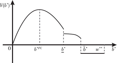
The Value Function Describes Case 1 of Proposition 6(b^*FC < b^*)

Figure 5

The Value Function Describes Case 2 of Proposition 6(b^* < b^*FC < b^*)

If China’s optimal choice of debt issuance corresponds to an inconsistent expectation of e^* that the US has chosen, then China adjusts e∗~ to ensure that finally China’s optimal debt issuance b^* is consistent with the e^* that the US has chosen.

Whether a Triffin dilemma arises for the US depends on the level of Chinese demand for reserve asset (w^*), compared to the safe debt capacity of the US (τ). All else equal, an increase in Chinese demand for safe asset or a decrease in the safe debt capacity activates the Triffin margin. The US then faces a choice between a low level of debt issuance at the boundary of the safety zone and a high level of debt issuance (min {b^FC, b}) in the instability zone.

Likewise, whether a Triffin dilemma arises for China depends on the level of Russian demand for reserve asset (w^**), compared to the safe debt capacity of China (τ^*). All else equal, an increase in the Russian demand for safe asset or a decrease in the safe debt capacity activates the Chinese Triffin margin. Then China faces a choice between a low level of debt issuance at the boundary of the safety zone and a high level of debt issuance (min{b^*FC, b^*}) in the instability zone.

In the following, I introduce the Proposition 7. Proposition 7 is a refinement of Proposition 5 and Proposition 6 combined. With generality, I consider the case in which e∗~ = 1 by default and then its value is adjusted to ensure the US, China and Russia are in equilibrium supposing they are off equilibrium for e∗~ = 1.

If none of the above situation happens, China will adjust the value of e∗~ until 1, 2 or 3 happens.

Next I prove Proposition 7. If the US encounters bad state, then the US either chooses full-commitment to the value of USD or a limited-commitment to the value of USD. If the US chooses full commitment, then its value function is V ^FC(b); if the US chooses limited commitment, then its value function is V (b).

The Chinese debt is also denoted by USD. If the US fully commits to the value of its debt or in the limited-commitment situation, the US chooses e^* = 1, then the value function for China is V^FC(b^*). If the US chooses e^* = eL∗ in the limited commitment situation, then the value function for China is V (b^*). In the later situation, whether China chooses its debt in the safety zone or in the instability/collapse zone determines its expectation towards the value of e^*.

Given e∗~ , according to the formula e^* = e × e∗~ , if the US devalues USD over RMB, then USD is devalued over RUB as well.

Suppose either the US commitment to the value of USD over RMB is limited and issues b^FC ∈ (0, b] in the safety zone, or the US fully commits to the value of USD over RMB and issues b^FC ∈ (0, b]. In the former situation, China’s value function is V(b^*) and issues b^* in the safety zone; in the latter situation, China’s value function is VF^C(b^*) and hence the Chinese debt issuance must be b^*FC ∈ (0, w^**]. Both situations are confirmation that the US is not devalued over RMB and hence USD is not devalued over RUB.

Suppose the US commitment to the value of USD is limited and issues either b or b^FC ∈ (b, b]. Hence, e = e_L. The following situations can happen for different parameter specifications:

1. the Chinese debt issuance is b^*FC ∈ (0, w^**].

2. China issues b* or b^FC ∈ (b^*, b^*].

However, in case 1, the expected value of e for China is e = 1. Only case 2 is consistent with the chosen value of e, which is e = e_L. If case 1 happens, apparently the US, China and Russia are off equilibrium. In this situation, China adjusts the value of e∗~ until the value of e∗~ reaches the value to make the US, China and Russia are on equilibrium. Therefore, Proposition 7 is proven. Q.E.D.

According to Caballero et al. (2017) and Farhi and Maggiori (2018, 2019), when the debt issuance of a country falls into the instability zone, then the country faces the possibility of a self-fulfilling confidence crisis. Such crisis is just the Triffin dilemma or Triffin event as featured in their models.

According to Proposition 7, if the US enters the instability zone, then China enters the instability zone; if the US commitment to the value of USD is full or the US stays in the safety zone given its commitment is limited, then the Chinese debt issuance is either of full commitment or in the safety zone with a limited commitment. Therefore, from this perspective, it can be said that the Triffin dilemma for the US and the Triffin dilemma for China are synchronized. It is all because the Chinese debt issued to Russia is denoted by USD.

The purpose of Chinese adjustment of e∗~ is to ensure that the US, China and Russia are in equilibrium. Improper value of e∗~ may make China’s expectation of whether USD is devalued over RUB inconsistent with the actual exchange rate adjustment of the US, and hence all players are not in equilibrium even though they try to maximize their respective payoffs. According to the formula e^* = e × e∗~ , the proper value of e^* given e can be calculated, which ensures that the US, China and Russia are in equilibrium after maximizing their respective payoffs, and then the corresponding value of e∗~ can be obtained from the formula accordingly. Based on the above rationale, we obtain the value range of e^* given various value of e that makes the US, China and Russia in equilibrium after maximizing their payoffs respectively.

If the US encounters bad state, to ensure the US, China and Russia are in equilibrium, e^* and hence e∗~=e∗e should fall into the following ranges in the situations e below respectively:

1. The US commitment to the value of USD over RMB is limited but issues b^FC in the safety zone. Then, I. given 1) w∗∗>2τ∗Rr∗¯ and τ∗≥maxRr∗¯28γ∗σ∗2,α∗λ∗Rr∗¯22γ∗σ∗2  or 2)  2τ∗Rr∗¯<w∗∗≤Rr∗¯−Rr∗¯2−8γ∗σ∗2τ∗2γ∗σ∗2 and α∗λ∗Rr∗¯22γ∗σ∗2<τ∗<Rr∗¯28γ∗σ∗2 if α∗λ∗<14, then by expecting that the US commitment to the value of USD over RMB is limited and e = 1, China devalues RMB over RUB until the RUB price of a USD falls into the following range:

   eL∗≤1−1−α∗γ∗σ∗22w∗∗2−2γ∗σ∗2τ∗Rr∗¯w∗∗−τ∗Rr∗¯α∗λ∗τ∗ (12)

   II. Given w∗∗>Rr∗¯−Rr∗¯2−8γ∗σ∗2τ∗2γ∗σ∗2,τ∗<Rr∗¯8γ∗σ∗2 and α∗>b∗¯w∗∗−b∗¯−τ∗Rr∗¯w∗∗−τ∗Rr∗¯b∗¯w∗∗−b∗¯+λ∗τ∗2γ∗σ∗2, then by expecting that the US commitment to the value of USD over RMB is limited and e = 1, China devalues RMB over RUB until the RUB price of a USD falls into the following range:

   eL∗≤1−1−α∗2γ∗σ∗2b∗¯w∗∗−b∗¯−2γ∗σ∗2τ∗Rr∗¯w∗∗−τ∗Rr∗¯α∗λ∗τ∗ (13)

2. The US fully commits to the value of USD over RMB and hence e = 1. China expects the US fully commits to the value of USD over RMB and e = 1. Because China has not adjusted the value of RMB over RUB, therefore the value of USD over RUB is kept as well. Hence, e^* = 1.

3. I. Given a) w∗>2τRr¯ and τ≥maxRr2¯8γσ2,αλRr2¯2γσ2 or b) 2τRr¯<w∗≤Rr¯−Rr¯2−8γσ2τ2γσ2  and  αλRr¯22γσ2<τ<Rr¯28γσ2 if αλ<14, once the US devalues USD over RMB, the devaluation extent for the US should satisfy:

   eL>1−(1−α)γσ22w∗2−2γσ2τRr¯w∗−τRr¯αλτ (14)

In this situation, the US commitment to the value of USD over RMB is limited and issues safe asset in the instability zone. China expects that the US commitment to the value of USD over RMB is limited and the US issues safe asset in the instability zone. Therefore, given 1) w∗∗>2τ∗Rr∗¯  and  τ∗≥maxRr∗¯28γ∗σ∗2,α∗λ∗Rr∗¯22γ∗σ2 or 2) 2τ∗Rr∗¯<w∗∗≤Rr∗¯−Rr∗¯2−8γ∗σ∗2τ∗2γ∗σ∗2  and  α∗λ∗Rr∗¯22γ∗σ∗2<τ∗<Rr∗¯28γ∗σ∗2 if α∗λ∗<14, China devalues RMB over RUB until the RUB price of a USD falls into the following range:

II. Given a) w∗>2τRr¯ and τ≥maxRr¯28γσ2,αλRr¯22γσ2 or b) 2τRr¯<w∗≤Rr¯−Rr¯2−8γσ2τ2γσ2  and  αλRr¯22γσ2<τ<Rr¯28γσ2 if αλ<14, once the US devalues USD over RMB, the devaluation extent for the US should satisfy

In this situation, the US commitment to the value of USD over RMB is limited and issues safe asset in the instability zone. China expects that the US commitment to the value of USD over RMB is limited and the US issues safe asset in the instability zone. Therefore, given w∗∗>Rr∗¯−Rr∗¯2−8γ∗σ∗2τ∗2γ∗σ∗2,τ∗<Rr∗¯8γ∗σ∗2 and α∗>b∗¯w∗∗−b∗¯−τ∗Rr∗¯w∗∗−τ∗Rr∗¯b∗¯w∗∗−b∗¯+λ∗τ∗2γ∗σ∗2, then China devalues RMB over RUB until the RUB price of a USD falls into the following range:

III. Given w∗>Rr¯−Rr¯2−8γσ2τ2γσ2,τ<Rr¯8γσ2 and α>b¯w∗−b¯−τRr¯w∗−τRr¯b¯w∗−b¯+λτ2γσ2,  once the US devalues USD over RMB, the devaluation extent for the US should satisfy

In this situation, the US commitment to the value of USD over RMB is limited and issues safe asset in the instability zone. China expects that the US commitment to the value of USD over RMB is limited and the US issues safe asset in the instability zone. Therefore, given 1) w∗∗>2τ∗Rr∗¯ and τ∗≥maxRr∗¯28γ∗σ∗2,α∗λ∗Rr∗¯22γ∗σ2 or 2) 2τ∗R∗∗¯<w∗∗≤Rr∗¯−Rr∗¯2−8γ∗σ∗2τ∗2γ∗σ∗2  and  α∗λ∗Rr∗22γ∗σ∗2<τ∗<Rr∗¯28γ∗σ∗2 if α∗λ∗<14, China devalues RMB over RUB until the RUB price of a USD falls into the following range:

IV. Given w∗>Rr¯−R2¯−8γσ2τ2γσ2,τ<Rr¯8γσ2  and  α>b¯w∗−b¯−τRr¯w∗−τRr¯b¯w∗−b¯+λτ2γσ2, once the US devalues USD over RMB, the devaluation extent for the US should satisfy

In this situation, the US commitment to the value of USD over RMB is limited and issues safe asset in the instability zone. China expects that the US commitment to the value of USD over RMB is limited and the US issues safe asset in the instability zone. Therefore, given w∗∗>Rr∗¯−Rr∗¯2−8γ∗σ∗2τ∗2γ∗σ∗2,τ∗<Rr∗¯8γ∗σ∗2 and α∗>b∗¯w∗∗−b∗¯−τ∗Rr∗¯w∗∗−τ∗Rr∗¯b∗¯w∗∗−b∗¯+λ∗τ∗2γ∗σ∗2, then China devalues RMB over RUB until the RUB price of a USD falls into the following range:

References

Caballero, R. J., Farhi, E., & Gourinchas, P. O. (2017). Rents, Technical Change, and Risk Premia - Accounting for Secular Trends in Interest Rates, Returns on Capital, Earning Yields, and Factor Shares. American Economic Review, 107, 5, 614–620.10.1257/aer.p20171036Search in Google Scholar
Caballero, R. J., Farhi, E., & Gourinchas, P. O. (2019). The Safe Assets Shortage Conundrum. Journal of Economic Perspectives, 31 (3), 29–46.10.1257/jep.31.3.29Search in Google Scholar
Calvo, G. (1988). Serving Public Debt: The Role of Expectations. American Economic Review, 78, 647–661.Search in Google Scholar
Farhi, E., & Maggiori, M. (2018). A Model of the International Monetary System. Quarterly Journal of Economics, 133(1), 295–355.10.1093/qje/qjx031Search in Google Scholar
Farhi, E., & Maggiori, M. (2019). China versus the United States: IMS Meets IPS. AEA Papers and Proceedings, 109, 476–481.10.1257/pandp.20191057Search in Google Scholar
© 2024 Rongyu Wang, Published by DeGryuter
This work is licensed under the Creative Commons Attribution 4.0 International License.
Articles in the same Issue
- Frontmatter
- Cumulative Tariff Cost Rate and Structure in the Global Value Chain: A Theoretical and Empirical Study
- Transportation Network Density, Domestic Market Integration and Excess Sensitivity of Household Consumption
- The Too-Big-to-Fail Premium in Tier-2 Capital Bonds and Additional Tier-1 Capital Bonds Primary Markets: Evidence from China
- Drivers of Portfolio Flows into Chinese Debt Securities Amidst China’s Bond Market Development