Inequality, Growth, and Congestion Externalities

Babatunde Aiyemo; AKM Mahbub Morshed

doi:10.1515/bejm-2020-0268

Artikel

Inequality, Growth, and Congestion Externalities

Babatunde Aiyemo und AKM Mahbub Morshed

Veröffentlicht/Copyright: 9. April 2021

Veröffentlicht von

Veröffentlichen auch Sie bei De Gruyter Brill

Manuskript einreichen Informationen für Autor*innen Erkunden Sie dieses Fachgebiet

Aus der Zeitschrift The B.E. Journal of Macroeconomics Band 21 Heft 2

Abstract

We describe and numerically simulate the aggregate and distributional properties of an endogenous growth model with an infrastructure externality which is subject to relative congestion. We show that the congested externality induces higher growth, greater inequality, labor/leisure trade-off ambiguities and an ineffective capital income tax for the government to achieve long-term redistribution goals. We demonstrate the economic implications of congestions in production and consumption externalities on the public to private capital ratio, growth and income distribution. Finally, we discuss alternative tax options for promoting inclusive growth.

Keywords: congestion; externalities; growth; inequality; public capital

JEL Classification: O1; O2; O3

Corresponding author: Babatunde Aiyemo, Department of Economics, Finance and Accounting, SUNY, Oneonta, USA, E-mail: aiyemob@oneonta.edu

Appendix

Appendix A. Sensitivity Analysis

In order to assess the sensitivity of our results to the complementarity of the productive inputs, we re-specify Eq. (1) in the form of a CES production function as follows;

(A1) Y j = A [ α K j − μ + ( 1 − α ) ( L j X j ) − μ ] − 1 μ

Where the elasticity of substitution is given by

(A2) ζ = 1 1 + μ

Optimizing on the productive inputs then produces the following equilibrium factor prices;

(A3) r = A − μ ( R ( 1 − α ) + α ) y μ + 1

(A4) w = A − μ z − μ ϵ α y ( 1 − l ) μ + 1

Our emphasis is therefore on the elasticity of substitution, ζ, which varies between zero, in the case where both factors are perfectly substitutable, and infinity, wherein they are perfect complements. Our strategy accordingly will be to calibrate the model for a low value of the elasticity of substitution, corresponding to ζ = 0.5, and a high equivalent, corresponding to ζ = 1.2.

As a benchmark, we evaluate the impact of congestion on inequality when infrastructure is financed using a non-distortionary lump-sum tax. The results are presented on Table A.9. On the upper panel, we present outcomes for the low elasticity state, while the lower panel shows the high elasticity equivalent following the expansion in infrastructure. The outcomes are consistent with the unitarily elastic case given that following the increase in θ, income inequality initially falls and then rises over time regardless of the nature of elasticity. Moreover, higher congestion levels consistently induce greater levels of economic growth and increases welfare inequality.

Table A.9:

Lump-sum tax-financed infrastructure, ζ = 0.5, 1.2.

ζ = 0.5
R	0	0.25	0.5
σ _k	−0.08	−0.3	−0.5
σ _u	0.4	1.8	1.6
σ _y(0)	−3.5	−3.2	−2.9
σ ̃ y	12.7	12.2	11.7
ψ	1.4	1.7	1.9
ζ = 1.2
σ _k	3.2	3	2.8
σ _u	6	5.6	5.2
σ _y(0)	−0.8	−1.3	−1.8
σ ̃ y	2.8	2.7	2.5
ψ	3.2	4.2	5.1

The sole pattern of divergence observable between high and low substitutability of factors arises from its impact on wealth inequality, which is negative when factors are highly substitutable, and positive when ζ = 1.2. Moreover, from the first column, it is apparent that this outcome is not due to congestion but is exacerbated by it.

Table A.10 produces calibration outcomes where the upgrade is financed by a capital income tax in both low and high substitutability conditions. The third and fourth rows confirm the results presented in the case of unitary elasticity, given that in all circumstances except where R = 0; ζ = 1.2, income inequality rises in the long run despite the activation of a capital income tax.

Table A.10:

Capital income tax-financed infrastructure, γ = 0.5, 1.2.

ζ = 0.5
R	0	0.25	0.5
σ _k	−0.14	−0.6	−0.8
σ _u	0	−0.5	−0.7
σ _y(0)	−23	−18	−15
σ ̃ y	3.6	4.7	5
ψ	1.3	1.6	1.8
ζ = 1.2
σ _k	4	3.6	3.3
σ _u	4.1	3.7	3.4
σ _y(0)	−5.5	−4.1	−3.7
σ ̃ y	−1.2	0.4	1.2
ψ	3	4	4.9

Accordingly, we highlight two distinct outcomes from this exercise. First is a reiteration of the underlying relationship between congestion, inequality and growth. Secondly, as the elasticity of substitution between capital and labor decreases, the degree of congestion required to abrade the redistributive efficacy of the capital income tax lessens.

Appendix B. The Linearized Matrix

Details of the linearized matrix given in Eq. (25) are indicated below;

a 11 = y ̃ z θ + y ̃ ( 1 − t w ) ( 1 − α ) 1 + t c η l ̃ 1 − l ̃ − ( 1 + R ( 1 − α ) − θ ) a 12 = y ̃ l ( 1 − t w ) ( 1 − α ) 1 + t c η l ̃ 1 − l ̃ − ( 1 + R ( 1 − α ) + 1 − t w 1 − α y ̃ z ̃ 1 + t c η 1 − l ̃ 2 a 21 = R ( 1 − α ) ( γ − t k ) + ( 1 − t k ) α + ( 1 − γ ) θ − 1 + ( 1 − t w ) ( 1 − α ) 1 + t c η l 1 − l y z − ε ( 1 − γ ) ( 1 − α ) a 11 z + G 3 1 H a 22 = ( 1 − t k ) ( R ( 1 − α ) + α ) y l − ( 1 − γ ) y l ( 1 + R ( 1 − α ) ) − 1 − t w 1 − α 1 + t c η 1 − l y l l + y 1 − l − ε ( 1 − γ ) ( 1 − α ) a 12 z + G 4 1 H

G 3 = h R c 1 − α 1 − t w y z l 1 − l + h η γ θ z y z − y z 2 G 4 = h R c 1 − α 1 − t w y l l + y 1 − l 2 + h η γ θ y l z

Appendix C. Distribution

C.1. Wealth

Combining Eqs. (8) and (20), we can express the evolution of relative capital k _i, defined as K i / K in the following way

(C1) k ̇ i = K ̇ i K i − K ̇ K k i = ω ( 1 − t w ) 1 − l i − l i η − τ y − ω ( 1 − t w ) 1 − l − l η − τ y k i

Which, given restrictions imposed by the transversality condition, is an unstable differential equation. Define;

G 1 ≡ ( 1 + t c ) Ω + ( 1 − t w ) ω ; G 2 ≡ ( 1 − t w ) ω − τ y

So that Eq. (C1) can be re-expressed as

k ̇ i ( t ) = G 2 − G 1 l i ( t ) + G 1 l ( t ) − G 2 k i ( t )

Or more conveniently as a linear deviation from the average wealth.

(C2) k ̇ i ( t ) = − G 1 l i ( t ) − l ( t ) + G 1 l ( t ) − G 2 k i ( t ) − 1

Where G ₁ ≥ G ₂. We will use the expression G _1x to indicate the derivative of G ₁ with respect to x. Setting k ̇ = 0 produces the following steady-state relationships;

(C3a) l ̃ i − l ̃ = l − G 2 G 1 ( k ̃ i − 1 )

(C3b) π i − 1 = 1 − G 2 G 1 l ̃ ( k ̃ i − 1 )

Linearizing Eq. (C2) around steady-state yields;

(C4) k ̇ i ( t ) = δ 1 k ̃ i − 1 z ( t ) − z ̃ + δ 2 k i ( t ) − k ̃ i

Where;

δ 1 ≡ ∂ k ̇ i ( t ) ∂ l d l d z + ∂ k ̇ i ( t ) ∂ z = G 1 z G 2 G 1 − G 2 z + G 2 l + G 1 l G 2 G 1 − G 2 l a 21 μ − a 22

δ 2 ≡ ∂ k ̇ i ( t ) ∂ k i = G 1 l − G 2

where, from the transversality condition, δ ₂ > 0.

In order to determine the sign of δ ₁, we note that G ₁ and G ₂ are both homogeneous in y. This means we can re-write the expressions as; G ₁ = Ay and G ₂ = By where A and B are given by;

A = ( 1 − t w ) ( 1 − α ) η + ( 1 − t w ) ( 1 − α ) ( 1 − l )

B = ( 1 − t w ) ( 1 − α ) ( 1 − l ) − τ

Then, the term

G 1 z G 2 G 1 − G 2 z

can be expressed as

G 1 , z G 2 − G 1 G 2 z G 1 = A B y − A y B ∂ y / ∂ z G 1 = 0

And similarly,

G 1 l G 2 G 1 − G 2 l = G 1 , l G 2 − G 1 G 2 l G 1 = A B y − A y B ∂ y / ∂ l G 1 = 0

Hence, the expression for δ ₁ reduces to

δ 1 = G 2 l a 21 μ − a 22

Fulfilling the transversality condition requires that G ₂/l > 0, while saddle-path stability requires that a ₂₁/(μ − a ₂₂) < 0. Accordingly, δ ₁ < 0.

Using the stable eigenvalue, the solution to Eq. (C4) is then given by

(C5) k i ( t ) − k ̃ i = δ 1 μ − δ 2 k ̃ i − 1 z ( t ) − z ̃

Note that since δ ₁ < 0, δ ₂ > 0 and the stable eigenvalue μ < 0, it therefore follows that δ ₁/(μ − δ ₂) > 0.

Given Eq. (C5), we now express relative capital in terms of its coefficient of variation

(C6a) σ k ( t ) = 1 + δ 1 μ − δ 2 z t − z ̃ σ ̃ k

(C6b) σ ̃ k = 1 + δ 1 μ − δ 2 z 0 − z ̃ − 1 σ k , 0

Dividing Eq. (C6a) by Eq. (C6b) yields Eq. (32) in the text, i.e.

σ k ( t ) = 1 + δ 1 μ − δ 2 z t − z ̃ 1 + δ 1 μ − δ 2 z 0 − z ̃ σ k , 0

C.2. Labor

Using Eq. (C3), relative wage can be expressed as;

(C7a) w i ( t ) − 1 = w L i ( t ) − L ( t ) w L ( t ) = l ( t ) 1 − l ( t ) 1 − G 2 G 1 l ̃ ( k ̃ i − 1 )

this implies

(C7b) σ w = l ( t ) 1 − l ( t ) 1 − G 2 G 1 l ̃ σ k

Taking the derivative of the right hand side and noting that dl/dR > 0. We obtain the following;

(C8a) d σ w d R = σ k 1 − l d l / d R 1 − l 1 − G 2 G 1 − l d G 2 / d R ︷ − − G 1 d l / d R ︷ + − l d G 1 / d R ︷ − G 1 l 2 ︸ − ︸ + + l d σ k / d R ︷ − 1 − l 1 − G 2 G 1 l ︸ −

The effect of congestion depends on whether the negative wealth effect (the second term) dominates the positive production substitution effect (the first term). Congestion increases leisure supply given the increased productivity of capital, which leads to an aggregate decrease in labor supply and an increase in the wage rate. Marginal product of labor increases, the gains of which are appropriated proportionally more by capital poor; however, the negative effect of congestion on wealth makes leisure expensive for capital rich agents such that they are compelled to supply more labor which invariably increases aggregate labor supply and lowers its productivity hence increasing wage inequality.

We also evaluate variations in the dispersion of wealth for changes in government’s share of output;

(C8b) d σ w d θ = σ k 1 − l d l / d θ 1 − l 1 − G 2 G 1 l − l d G 2 / d θ ︷ + − G 1 d l / d θ ︷ − − l d G 1 / d θ ︷ + G 1 l 2 ︸ + ︸ − + l d σ k / d θ ︷ + 1 − l 1 − G 2 G 1 l ︸ +

The sign directions above indicate that although the increased government share has a productivity augmenting impact for labor, this is appropriated by all agents and since aggregate labor supply increases due to the stimulus, the dispersion in labor income is widened by the expansionary policy thus leading to the negative sign on the first component. However, the expansion implies that capital rich agents now supply even less labor given that they now face a more dispersed relative capital edge which consequently compresses the wage dispersion, hence the positive sign on the second component. When compared with the result from Eq. (C8a), congestion acts in a converse direction to policy, so that its impact in a growing economy would be to decrease the extent of variation associated with wealth inequality during a fiscal expansion and increase it during a contraction given the pure factor supply effect.

C.3. Welfare

The welfare of individual i is defined as their utility function evaluated along the equilibrum growth path. Accordingly, integrating Eq. (7a) for agent i at the commencement of period 0 and setting h = 0 produces the following;

(C9a) W i = 1 γ [ ( C j / K i ) l i η ] γ β − ψ γ K i , 0 γ

The equivalent for aggregate welfare is given by;

(C9b) W = 1 γ [ ( C / K ) l η ] γ β − ψ γ K 0 γ

And from Eq. (13), we obtain;

(C10) C i K i = Ω l i k i

Accordingly, substituting Eq. (C10) into Eq. (C9a) for C _i/K _i; Eq. (13) into Eq. (C9b) for C/K, and dividing Eq. (C9a) by Eq. (C9b) expresses relative welfare in terms of the labor/leisure choice of individual i thus;

(C11) W i W ≡ x i = l i l ( 1 + η ) γ

Noting that l _i/l = π _i, we substitute for π _i from Eq. (C3b) into Eq. (C11) to obtain

(C12) x i = 1 + 1 − G 2 G 1 l ̃ ( k ̃ i − 1 ) ( 1 + η ) γ

Its monotonic transformation yields the metric u for evaluating relative welfare, defined as follows

(C13) x i 1 γ ( 1 + η ) ≡ u = 1 + ϕ ( k ̃ i − 1 ) ;

where

(C14) ϕ = 1 − G 2 G 1 l ̃

Accordingly, the coefficient of variation of relative welfare is given by

(C15) σ u = ϕ σ ̃ k

Given the empirical motivation, much of our analysis imposes the restriction h = 0. However, for h ≠ 0, we will have the following modification to Eq. (C11)

(C16) W i W ≡ x i = k i h R c η γ l i l ( 1 + η ) γ

In which case, Eq. (C13) is expressed as

(C17) x i 1 γ ( 1 + η ) ≡ u = k i P + ϕ k i P ( k ̃ i − 1 ) ;

where P = hR _c η/(1 + η). From Eq. (C14) and (C15), the impact of an expansionary fiscal policy in the presence of congestion can then be derived as being

(C18) d σ ̃ u d θ = σ ̃ k d G 2 d θ ︷ + − [ G 1 d l d θ ︷ − − l d G 1 d θ ︷ + ] G 1 l 2 ︸ + + d σ ̃ k d θ ︷ + 1 − G 2 G 1 l ̃ ︸ +

(C19) d σ ̃ u d R = σ ̃ k d G 2 d R ︷ − − [ G 1 d l d R ︷ + − l d G 1 d R ︷ − ] G 1 l 2 ︸ − + d σ ̃ k d R ︷ − 1 − G 2 G 1 l ̃ ︸ −

The above implies that the fiscal stimulus unambiguously increases welfare dispersion while congestion decreases it so that actual dispersion of welfare is typically contained between both margins. Along the transition path welfare inequality remains unchanged so that steady-state dispersion levels are instantly visible upon policy change.

Appendix D. Excludable Public Capital

Extending the model to account for excludability per Ott and Turnovsky (2006), implies modifying Eq. (1b) such that the externality is now made up of two components; one which is excludable, and the other which is not. To restrict our focus to the publicly provided externality, we set ɛ = 1 and denote the productivity associated with the excludable part of the publicly provided externality as σ. The composite externality X _j then assumes the form;

(D1) X j = K E σ K j K R 1 K N 1 − σ K j K R 2

Where K _E and K _N represent the aspect of public capital that are excludable and non-excludable respectively. R1 and R2 are also now the extent of congestion associable with the excludable and non-excludable externality.

Output as perceived by the jth producer is now given by

(D2) Y j = A K E σ ( 1 − α ) K N ( 1 − σ ) ( 1 − α ) K j K R 1 ( 1 − α ) K j K R 2 ( 1 − α ) L j ( 1 − α ) K j α

With the equilibrium marginal product of capital being analogous to Eq. (5) as

(D3) r = ( ( R 1 + R 2 ) ( 1 − α ) + α ) y

The consumer now maximizes a Hamiltonian which includes two types of publicly availed resources, where the excludable aspect of this externality imposes a user fee, p. Hence, the consumer has to optimize on the quantity of this excludable resource required to maximize utility. This leads to an extra first-order condition;

(D4) Ω K E a ≡ ∂ Y j ∂ K E = σ ( 1 − α ) Y j K E D = p

Here K E D now represents the quantity of the excludable capital that the consumer demands. In equilibrium, this quantity demanded will equal the quantity supplied. Taking the quantity as a proportion of output, K _E = θ ₁ Y, it then becomes clear that the user fee is a fixed rate

(D5) p = σ ( 1 − α ) θ 1

Note also that the equilibrium user fee is independent of the extent of congestion in the economy. By this token, the sole difference between the user fee and a flat tax on output is in the voluntary opt-in associated with the user fee. It is however also the case that the productive nature of public capital makes its take-up essentially guaranteed from the perspective of the profit-maximizing producer. It therefore naturally follows that the aggregate and distributional consequences of such an externality in the decentralized economy are also fully described using the budget constraint from Eqs. (8) and (16) where p may now be a construed as a component of the proportional tax on output, i.e. τ.

See Figure E.4.

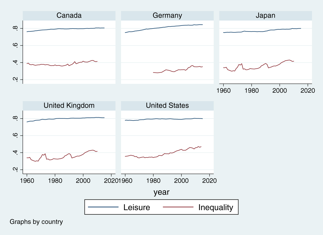
$Figure E.4: Leisure hours and income inequality. Income inequality is evaluated using the fraction of output accruing to the top decile. Source: PWT and WIID.$

Figure E.4:

Leisure hours and income inequality. Income inequality is evaluated using the fraction of output accruing to the top decile. Source: PWT and WIID.

References

Andres, L., D. Biller, and M. H. Dappe. 2014. “Infrastructure Gap in South Asia: Inequality of Access to Infrastructure Services.” World Bank Policy Research Working Paper 7033.Suche in Google Scholar

Arrow, K. J., and M. Kurz. 1970. “Optimal Growth with Irreversible Investment in a Ramsey Model.” Econometrica: Journal of the Econometric Society 331–44. https://doi.org/10.2307/1913014.Suche in Google Scholar

Aschauer, D. A. 1989. “Is Public Expenditure Productive?” Journal of Monetary Economics 23 (2): 177–200. https://doi.org/10.1016/0304-3932(89)90047-0.Suche in Google Scholar

Barro, R. J. 1990. “Government Spending in a Simple Model of Endogenous Growth.” Journal of Political Economy 98: S103–25. https://doi.org/10.1086/261726.Suche in Google Scholar

Barro, R., and X. Sala-i-Martin. 1992. “Public Finance in Models of Economic Growth.” The Review of Economic Studies 59: 645–61. https://doi.org/10.2307/2297991.Suche in Google Scholar

Bom, P., and J. Ligthart. 2010. What Have We Learned from Three Decades of Research on the Productivity of Public Capital? Mimeo: Tilburg University.Suche in Google Scholar

Calderon, C., and L. Serven. 2014. “Infrastructure, Growth, and Inequality: An Overview.” In Policy Research Working Paper; No. 7034. Washington, DC: World Bank Group.Suche in Google Scholar

Caselli, F., and J. Ventura. 2000. “A Representative Consumer Theory of Distribution.” The American Economic Review 90: 909–26. https://doi.org/10.1257/aer.90.4.909.Suche in Google Scholar

Chatterjee, S., and S. Ghosh. 2011. “The Dual Nature of Public Goods and Congestion: The Role of Fiscal Policy Revisited.” Canadian Journal of Economics 44: 1471–96. https://doi.org/10.1111/j.1540-5982.2011.01681.x.Suche in Google Scholar

Chatterjee, S., and S. Turnovsky. 2012. “Infrastructure and Inequality.” European Economic Review 56: 1730–45. https://doi.org/10.1016/j.euroecorev.2012.08.003.Suche in Google Scholar

Cooley, T. F. 1995. Frontiers of Business Cycle Research. Princeton, NJ: Princeton University Press.Suche in Google Scholar

Edwards, J. H. Y. 1990. “Congestion Function Specification and the ‘Publicness’of Local Public Goods.” Journal of Urban Economics 27: 80–96. https://doi.org/10.1016/0094-1190(90)90026-j.Suche in Google Scholar

Eicher, T., and S. J. Turnovsky. 2000. “Scale, Congestion and Growth.” Economica 67: 325–46. https://doi.org/10.1111/1468-0335.00212.Suche in Google Scholar

Fisher, W. H., and S. Turnovsky. 1998. “Public Investment, Congestion and Private Capital Accumulation.” The Economic Journal 108: 399–413. https://doi.org/10.1111/1468-0297.00294.Suche in Google Scholar

Futagami, K., Y. Morita, and A. Shibata. 1993. “Dynamic Analysis of an Endogenous Growth Model with Public Capital.” The Scandinavian Journal of Economics 95: 607–25. https://doi.org/10.2307/3440914.Suche in Google Scholar

Garcia-Penalosa, C., and S. J. Turnovsky. 2006. “Growth and Income Inequality: A Canonical Model.” Economic Theory 28: 25–49. https://doi.org/10.1007/s00199-005-0616-7.Suche in Google Scholar

Garcia-Penalosa, C., and S. J. Turnovsky. 2007. “Growth, Income Inequality and Fiscal Policy: What Are the Relevant Tradeoffs?” Journal of Money, Credit, and Banking 39: 369–94. https://doi.org/10.1111/j.0022-2879.2007.00029.x.Suche in Google Scholar

Guvenen, F. 2006. “Reconciling Conflicting Evidence on the Elasticity of Intertemporal Substitution: A Macroeconomic Perspective.” Journal of Monetary Economics 53: 1451–72. https://doi.org/10.1016/j.jmoneco.2005.06.001.Suche in Google Scholar

Kaldor, N. 1957. “A Model of Economic Growth.” The Economic Journal 67 (268): 591–624. https://doi.org/10.2307/2227704.Suche in Google Scholar

Kuznets, S. 1955. “Economic Growth and Income Inequality.” The American Economic Review 45 (1): 1–28.Suche in Google Scholar

Klenert, D., L. Mattauch, O. Edenhofer, and K. Lessmann. 2018. “Infrastructure and Inequality: Insights from Incorporating Key Economic Facts about Household Heterogeneity.” Macroeconomic Dynamics 22 (4): 864–95. https://doi.org/10.1017/s1365100516000432.Suche in Google Scholar

Lansing, K. 1995. “Is Public Capital Productive? A Review of the Evidence.” Economic Commentary, Cleaveland, Ohio: Federal Reserve Bank of Cleveland.Suche in Google Scholar

Ott, I., and S. Turnovsky. 2006. “Excludable and Non-excludable Inputs: Consequences for Economic Growth.” Economica 73: 725–48. https://doi.org/10.1111/j.1468-0335.2006.00506.x.Suche in Google Scholar

Pintea, M., and S. Turnovsky. 2006. “Congestion and Fiscal Policy in a Two-Sector Economy with Public Capital: A Quantitative Assessment.” Computational Economics 28: 177–209. https://doi.org/10.1007/s10614-006-9038-2.Suche in Google Scholar

Romer, P. M. 1986. “Increasing Returns and Long-Run Growth.” Journal of Political Economy 94: 1002–37. https://doi.org/10.1086/261420.Suche in Google Scholar

Straub, S. 2008. Infrastructure and Development: A Critical Appraisal of the Macro Level Literature. Washington, D.C.: The World Bank.10.1596/1813-9450-4590Suche in Google Scholar

Turnovsky, S. J. 2000. Methods of Macroeconomic Dynamics. Cambridge Massachusetts: MIT Press.Suche in Google Scholar

Received: 2019-12-14

Revised: 2021-03-18

Accepted: 2021-03-20

Published Online: 2021-04-09

Sie haben derzeit keinen Zugang zu diesem Inhalt.

Artikel in diesem Heft

https://doi.org/10.1515/bejm-2020-0268

Schlagwörter für diesen Artikel

congestion; externalities; growth; inequality; public capital