Radiogenic heating in comets: A computational study from an astrobiological perspective

Thaskeena Angeveettil Abubacker; Nalin Chandra Wickramasinghe; Godfrey Louis

doi:10.1515/astro-2025-0011

Article Open Access

Radiogenic heating in comets: A computational study from an astrobiological perspective

Thaskeena Angeveettil Abubacker , Nalin Chandra Wickramasinghe and Godfrey Louis

Published/Copyright: May 23, 2025

Published by

Become an author with De Gruyter Brill

Submit Manuscript Author Information Explore this Subject

From the journal Open Astronomy Volume 34 Issue 1

Abstract

Over the past two decades, interstellar dust and cometary material have been found to include a significant content of organic and biogenic molecules. This possibly hints towards a genesis of life in cometary bodies, with comets acting as carriers of microbial life throughout the galaxy. We describe here a computational study of the role of radiogenic heating due to 26 Al in the thermal evolution of a cometary interior and thereby delineate zones with possible liquid water content. Thermal evolution calculations are carried out for comets possessing various radii, starting from an initial accretion phase to some 100 million years after the completion of accretion. Our computation shows that comets with radius 6 km and higher can have liquid water interior regions and hence can support zones where microbes can survive. Such microbial survival zones are traced out as regions where the temperature rises above the melting point of water ice and later remain below a sterilizing temperature. The active time available for possible microbial multiplication is also determined. Computations also show that survival zones are not generally found at the centres of comets but at varying radial distances from the centre, depending on the radius of the comet.

Keywords: comet; radiogenic heating; astrobiology; microbial survival zone

1 Introduction

The investigation into the organic nature of interstellar dust initiated by Fred Hoyle and one of the present authors (NCW) in the 1970s marked a pivotal shift in our understanding of the cosmos (Hoyle and Wickramasinghe 1982, 1985, 2000, Wickramasinghe 2010). Challenging the entrenched terrestrial-based Oparin–Haldane model, the discovery of vast quantities of organic molecules and polymers in the universe hinted at an astronomical origin of life, a concept increasingly supported by new astronomical spectroscopy (Hoyle et al. 2015).

The transformative observations of Comet Halley in 1986 shattered the conventional view of comets as mere “dirty snowballs”. The encounter revealed a complex nucleus, debunking the traditional model and sparking a re-evaluation of cometary composition (Wickramasinghe and Allen 1986). Subsequent missions, notably the Rosetta probe’s exploration of Comet 67P/CG, provided evidence of carbon-bearing compounds on the nucleus of the comet (Capaccioni et al. 2015), which could, in part, be a relic of biological activity within the comet (Hoyle et al. 1984). Recent advancements, including laboratory studies of carbonaceous asteroids (Hoover et al. 2021) and the discovery of giant comets being active at large heliocentric distances (Wickramasinghe 2022), offer further new insights into the potential for microbial habitats within cometary interiors.

The profuse emission of gas and dust occurring for some comets in the cold depths of space far beyond the orbit of Jupiter, where both thermal evaporation and surface detonation of chemical processes would be ruled out, was stressed some years ago by Wickramasinghe, Hoyle, and Lloyd (Wickramasinghe et al. 1996). The first such phenomenon was discovered for Comet Hale–Bopp erupting at a distance of 6.5AU in 1983/84 long before it had reached perihelion in April 1997. More recently, in 2015 Comet Lovejoy, erupting much closer to the sun at 1AU distance, emitted vast amounts of sugar and ethyl alcohol (Biver et al. 2015). The simultaneous occurrence of these two molecules points towards the possibility of a fermentation process, which may take place in subsurface liquid domains of the comet, conducive to microbial metabolism.

It is often argued that life originated on Earth itself, facilitated by favourable chemical conditions present on early Earth (Pearce et al. 2017). However, these same mechanisms could potentially operate on a multitude of exoplanets (Rimmer et al. 2018), suggesting that life might arise elsewhere under similar conditions. Additionally, life may even be transported across different regions of the universe, spreading through various suggested mechanisms, including directed panspermia (McKay et al. 2022) and possible seeding through comet fragments (Louis and Kumar 2006).

In a recent study, Moody et al. (2024) reported that the Last Universal Common Ancestor (LUCA), with a genome comparable to modern prokaryotes, lived on Earth about 4.2 billion years ago. This age is comparable to the geological age of Earth, and it shows that life appeared remarkably quickly after the planet’s formation. This surprisingly rapid appearance of life on Earth can be interpreted in two ways: either a rapid abiogenesis has taken place on early Earth, or the LUCA or its evolutionary predecessor arrived here from space. If the first option is correct, it implies that life must be common in the universe, as it can readily emerge on Earth-like planets under suitable conditions. The second option suggests that life took its time to originate in a potentially favourable extraterrestrial environment before being transported to suitable planets like Earth. The exact mechanism of abiogenesis, whether it occurred on Earth or elsewhere, remains yet to be known.

Impact ejection events (Stoffler et al. 2007) and space dust collision (Berera 2017) are possible mechanisms by which microorganisms or their spores can escape from life bearing planets. Spores of microbes are now known to survive extreme conditions (Nicholson et al. 2000). A small but significant fraction of such spores may be transported to interstellar regions and possibly get incorporated into newly forming comets (Wallis and Wickramasinghe 2004, Valtonen et al. 2008). If the comet interior undergoes radiogenic heating, which may produce liquid water, then in the presence of chemical nutrients, such spores have a chance to germinate and undergo biological amplification (Wickramasinghe et al. 2009). The organic compounds present in comets (Ehrenfreund et al. 2011, Venkataraman et al. 2023, Hanni et al. 2022) may serve as nutrients for the growth of chemotrophic microbes.

This study is directed at determining whether appropriate thermal conditions and liquid water exist to facilitate the survival and multiplication of microorganisms in comets. More specifically, we aim to find microbial survival zones (MSZs) inside comets by computing the time-dependent thermal profiles of comets under radiogenic heating. Such zones in comets are defined here as having the presence of liquid water for finite lengths of time and not reaching sterilizing temperatures at a later stage. The comets examined in this study are assumed to be sufficiently distant from their host star, allowing us to neglect the effects of stellar heating and the resulting outgassing.

In the case of small bodies like comets, only short-lived isotopes have importance for radiogenic heating (Merk and Prialnik 2003). The radioactive isotope 26 Al with a comparatively short decay time of 1.06 × 1 0 6 years has earlier been recognized as a potential heat source (Suess and Urey 1956). The presence of 26 Al in the small solar system bodies was confirmed by the detection of interstellar 1.809 MeV gamma rays (Diehl et al. 1995) and 26 Mg enhanced abundance found in Ca-Al-rich inclusions of meteorites (MacPherson et al. 1995). Such evidence points towards an interstellar isotopic ratio of 26 Al/ 27 Al ∼ 5 × 1 0 − 5 , implying an initial mass fraction of 7 × 1 0 − 7 in solar nebula dust, and an order of magnitude less, on average, in objects like comets, for which the time of aggregation did not exceed a few million years (Lugmair and Shukolyukov 2001).

Ellsworth and Schubert (1983), Prialnik et al. (1987), Haruyama et al. (1993), Yabushita (1993), De Sanctis et al. (2001), Irvine et al. (1980), Wallis (1980), Prialnik et al. (2004), and Rosenberg and Prialnik (2007) have developed a range of theoretical models in order to understand the effect of radiogenic heating due to short-lived radioactive nuclide 26 Al in comets, asteroids etc.

For the ease of computation, in most of the previous studies, accretion was assumed to be instantaneous, neglecting any thermal consequences. But, timescale of radiogenic heating and time taken for accretion are comparable. So, our present modelling seeks to combine the earlier thermal models with the additional process of dynamical accretion. Omitting this process is tantamount to avoiding the period in a comet’s history when the radionuclide 26 Al was probably the most potent heat source.

In this work, we shall mainly focus on the outcome of radiogenic heating in comets, starting with an accretion phase, and then attempt to identify possible MSZs inside the comet. The modelling discussed in this article will seek to provide a justification for certain observations mentioned earlier that would otherwise remain poorly understood.

2 Methodology

2.1 Thermal profile calculation

To study the effect of radiogenic heating on the thermal profile of a comet nucleus, the physical equations and models have to be adjusted for specific calculations. For this, the comet nucleus can be divided into elements via a grid and assuming a homogeneous lumped system approximation for each such element.

According to Fourier’s law,

(1) F = − K ∇ T ,

where F is the heat flux, K is the conduction coefficient, and T is the temperature. If all substances of volume fraction X i and conduction coefficient K i are distributed evenly in the system, then the effective conduction coefficient is

(2) K = Σ X i K i .

When all fluxes through a lumped system are combined, we obtain the heat transfer equation

(3) − ∇ . F + Q = ρ c p ∂ T ∂ t ,

where ρ is the bulk density, c p is the specific heat capacity, and Q is the rate of energy release. The rate of heat produced due to radioactivity in a volume element Δ V is the only term included in Q . Then, the heat transport equation inside the comet nucleus is

(4) ρ c p ∂ T ∂ t = ∇ . ( K ∇ T ) + Q .

Assuming a uniform composition for the comet, K can be independent of r and the temperature dependence of K is considered negligible (Hahn and Özşik 2012). Hence, the conductivity is taken as a constant.

Since it is difficult to model a non-spherical object (Prialnik et al. 2004), spherical symmetry is assumed for simplicity and a spherical polar coordinate system is used. Since the heat source (radioactive material) is evenly distributed throughout the comet, lateral conduction can be avoided and heat conduction is assumed to occur only along the radial direction. Now, the problem is reduced to a 1D problem in spherical polar coordinates, which requires a single dimensional parameter – the effective radius r . The aforementioned equation becomes

(5) ρ c p ∂ T ∂ t = K r 2 ∂ ∂ r r 2 ∂ T ∂ r + Q ,

where T ( r , t ) is the temperature at a radial distance r from the centre at time t . Now, define a parameter thermal diffusivity α = K ρ c p

(6) ∂ T ∂ t = α ∂ 2 T ∂ r 2 + 2 α r ∂ T ∂ r + q ρ c p .

Eq. (6) is a linear, non-homogeneous, time-dependent second-order partial differential equation. Since heat conduction is confined to a radial direction only, the aforementioned grid discretisation can be replaced by concentric hollow spheres separated by a distance Δ r . All points of each sphere will possess same temperature at a time t .

Finite difference method is used to solve the aforementioned equation. The most common and simplest scheme is the “explicit method”. This has the disadvantage that the time step is restricted by the Courant–Friedrichs–Levy condition, Δ t ≤ ( Δ r ) 2 ∕ 2 α . Thus, time step may become too small when a fine mesh is required in order to resolve sharp temperature variations. Moreover, in this particular problem, while fixing the time step, it should be done in such a way that Δ t should be greater than or equal to the time taken for the transmission of the effect of change in temperature that happened at the centre to the surface of the comet. Therefore, we use the Crank–Nicholson scheme, which is a modified form of the so-called implicit scheme. This procedure has the advantage of being second-order accurate in time and unconditionally stable for all values of the time step. To perform Crank–Nicholson scheme, the initial value of temperature at any point, the surface and central temperatures at any time must be known.

The radiation temperature of interstellar space is 3.5 K (Allen 1976). Cometary formation is likely to have taken place in an environment of temperature below 15 K. Then, the surface temperature will only be slightly different from the ambient regional temperature (Yabushita and Wada 1988), approximately 20 K. The value of central temperature at each time step is explicitly calculated at the beginning of the time step. The initial temperature at any point can be obtained as an end product of accretion phase analysis.

2.2 Accretion phase analysis

We are assuming an accretion scenario in which any stochastic collision may result in a coalescence. To start with, we assume that there is a seed body of radius 500 m. The seed body can accumulate dust grains from its surroundings and grow in size. One of the suitable mathematical approaches to deal with such a situation is, by employing moving boundary condition on the spherically symmetric heat transport Eq. (6). Let R p 0 be the initial radius of the seed body at the onset of accretion and R p max be the final radius. Fixing the time taken for accretion t accr as being of the order of a few million years is considered to be reasonable (Weidenschilling 1988). A linear accretion law R p ( t ) = R p 0 + ( ( R p max − R p ( 0 ) ) ∕ t accr ) t is assumed in most of the studies (Merk et al. 2002).

The temperature of the ambient nebula T N is the initial temperature of the accreting particles. It is already shown that (Wetherill and Stewart 1989) the impact heating power is smaller than the total energy radiated per unit surface area per unit time by about two or three orders of magnitude. Thus, the temperature of the surface material will equilibrate with that of newly accreted material, which is T N . For this reason, surface temperature can be approximated to T N , a constant value at any time (i.e. during and after accretion phase). In short, the assumption is that, thermodynamically, the accreting comet is embedded in a large tank of temperature T N . Then, the following equation inherently include the accretion:

(7) T ( R p ( t ) , t ) = T N .

We start the analysis by imposing a zero-flux boundary condition at the centre at any time and with a seed body of radius R p 0 , which has a uniform temperature distribution, T N , i.e.,

(8) T ( r , t 0 ) = T N ,

(9) ∂ T ∂ r r = 0 = 0 ,

(10) T ( R p ( t ) , t ) = T N ,

are the initial and boundary conditions, respectively. It is a moving boundary-value problem.

In order to solve such problems, usually, it is seen that the boundary of the domain is fixed at a constant value 1, using dynamical scaling of the radial coordinates by applying coordinate transformation. But such a scaling procedure does not resolve finer spatial variations in temperature as the comet grows in size due to accretion. Instead of a fixed number of strips with growing strip size, we choose a method in which, an additional number of strips with equal width as per growth rate are added in each time step till the completion of accretion. To accomplish this, we fix the number of strips and time steps in such a way that the number of strips attached to the parent body in each time step should be an integer, and also the time step and strip size are restricted by Courant–Friedrichs–Levy condition, δ t ≤ ( Δ r ) 2 ∕ 2 α . However, it should be noted that both the aforementioned conditions turned out to be difficult to meet at the same time. So, we switched to the alternative Crank–Nicholson method (which is unconditionally stable for all values of time steps) itself in accretion time analysis. To perform the Crank–Nicholson method a minimum number of strips are required. Until then, explicit method is used.

The accretion phase and post-accretion phases were analysed separately. Numerical calculations were carried out using our computer program developed in the Python language.

2.3 Assumptions and limitations

The comets do not have to be spherical in shape. However, for mathematical simplicity in our current model, we assume spherical symmetry. Therefore, only radial heat conduction could be accounted. Our model comets are assumed to have a uniform density and composition with temperature-independent thermal conductivity and specific heat capacity.

Assuming a uniform composition leads to radius-independent values for effective ρ , k , and c p . A uniform distribution of radioactive material is also considered. The temperature dependence of k and c p is also not considered. The calculations are carried out without considering the various pore properties in detail.

There are several involved methods to calculate the effective thermal conductivity of porous matrix (Marboeuf et al. 2012, Prialnik et al. 2004, Shoshany et al. 2002). In this study, as an approximation, we have only used volume-weighted sum in which pore portions are also taken as a component with extremely low conductivity ( ∼ 0.001 W m − 1 K − 1 ).

In order to avoid the artifacts and instabilities in simulations, a large value of specific heat capacity is needed to be assigned to pores (Kaviany 2012). Therefore, pores are assumed to have a specific heat capacity of the order of 1 0 4 and a density of zero.

We assume that the pressure within the interior of the comet nucleus is above the triple-point value (6.12 mbar), so that direct sublimation of water ice can be neglected.

In low-gravity environments, such as in the interior of comets, buoyancy forces are expected to be small and the convective process of mass transfer and consequent heat transfer may not be significant in comparison with conduction heat transfer. Hence, in the present model, possible mass flow within the comet is neglected and liquid water is expected to remain stationary to a great extent. Consequently, the heat transfer is assumed to be taking place only due to conduction and not due to convection.

2.4 Numerical values of parameters

The models considered in this study differ only in radius, which varies in the range 5 ≤ R ≤ 100 km and all other free parameters are fixed such that ice-dust ratio at 2:1 and porosity at 50%. The effective values of density, specific heat capacity, and thermal conductivity are taken as the volume-weighted sum. The numerical values of parameters (Prialnik et al. 2004) considered in this study are summarized in Table 1.

Table 1

Numerical values of the parameters

Parameter	Numerical value	Units
c p of dust	∼ 800	J kg − 1 K − 1
c p of ice	2,000	J kg − 1 K − 1
c p of liquid water	4,184	J kg − 1 K − 1
ρ of ice	910	kg m − 3
ρ of water	1,000	kg m − 3
ρ of dust	1,400	kg m − 3
K of dust	∼ 0.1–4.0	W m − 1 K − 1
K of ice	2.5	W m − 1 K − 1
K of water	0.6	W m − 1 K − 1
L f of water ice	334	kJ kg − 1

Even though the thermal parameters can take a range of values as shown in table, in this study, we are discussing the results for temperature-independent parameter values K dust = 1.1 W m − 1 K − 1 and hence an effective conductivity of 1.01 W m − 1 K − 1 , effective specific heat capacity of 3,290 J kg − 1 K − 1 , and effective density of 540.75 kg m − 3 . The values after melting are also chosen accordingly.

The only radioactive element considered is 26 Al, which has a half-life of 0.74 Myr. The initial mass fraction in solar nebula dust is 7 × 1 0 − 7 (MacPherson et al. 1995). The accretion time analysis starts with this concentration. A fully formed comet will have an 26 Al mass fraction, which is left over after radioactivity during accretion time (Lugmair and Shukolyukov 2001).

3 Results and discussions

3.1 Accretion phase

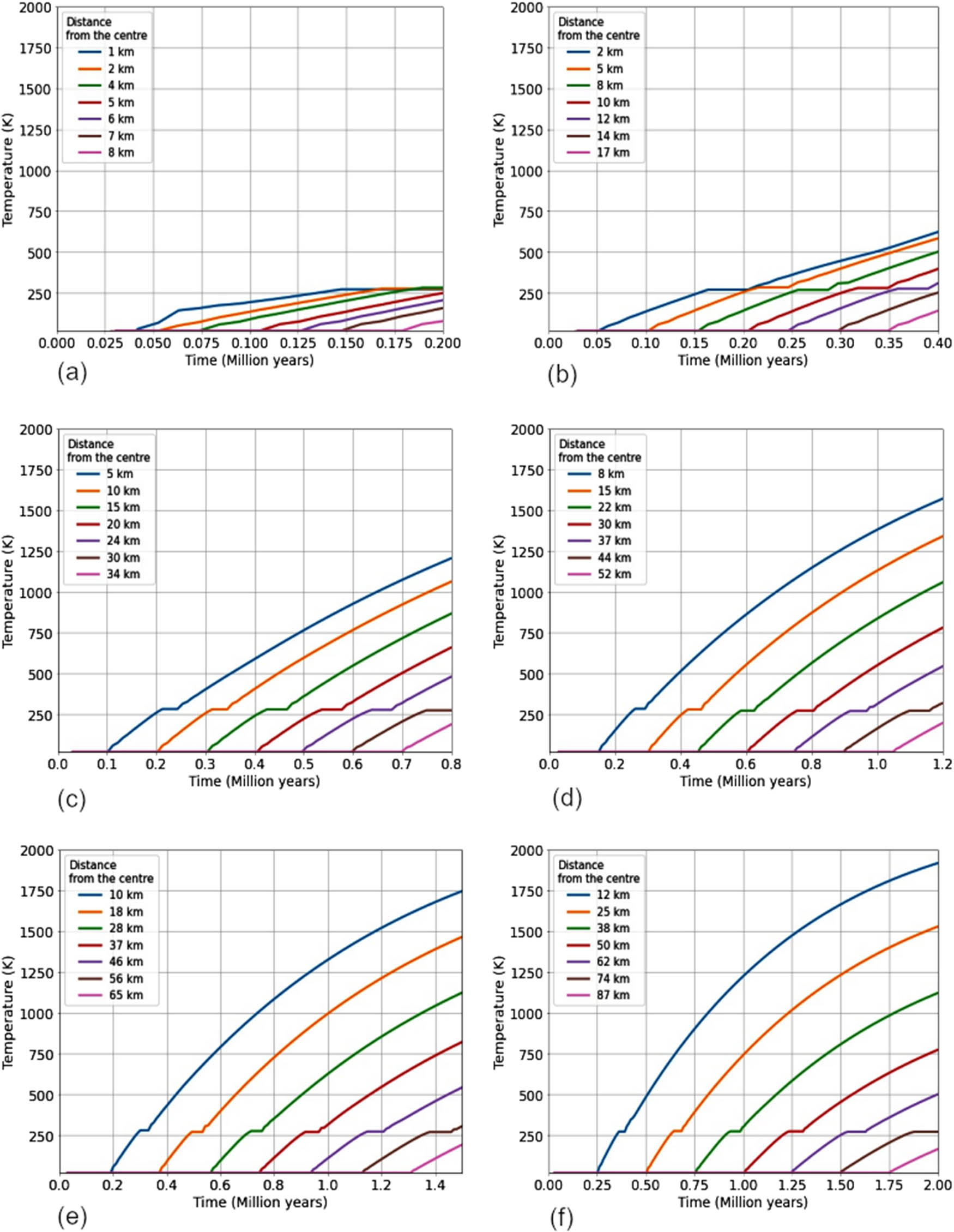
Figure 1 shows the temperature profile at distinct radial distances from the centre during accretion for comet models with different radii. Each curve has a different starting point in the x -axis. This is because of the delayed addition of material to the growing comet. The temporary pause in rising temperature in most curves is due to the latent heat of ice melting.

Figure 1

Time-dependent thermal profile of comets with different radii (a) 10 km, (b) 20 km, (c) 40 km, (d) 60 km, (e) 75 km, and (f) 100 km during accretion. Different coloured lines indicate specific distances from the centre of the accreting comet. The temporary pause in the rising trend of the temperature profile is due to the melting of water ice in that region during the corresponding time.

While solving the partial differential equation using the finite difference method, it is observed that the solution often exhibits oscillatory behaviour in the first two to three time steps, which then disappears. The effect of this behaviour is negligible in the case of larger comets. However, this computational anomaly is a little bit prominent in the case of comets with radius ≤ 10 km, in which the number of time steps are fewer during accretion time thermal analysis.

Figure 2a is the post accretional spatio-temporal variation of comet of radius 40 km, without doing an accretion time thermal analysis. Instead, we took the initial central temperature as 100 K and merely considered exponentially decreasing initial temperatures along the radius. However, Figure 2(b) shows the post-accretional spatio-temporal variation of temperature of a same-size comet, in which accretion time thermal analysis is carried out, and which is entirely different from Figure 2(a). It is found that, considering accretion gives a more realistic picture of temperature profile. It is seen that the temperature profile does not take any particular functional form at the time of completion of accretion. Looking at the Figure 3 itself, it is seen that the profile shows a slow variation in the central regions and fast variation away from the centre.

Figure 2

The computed colour map of the post-accretional thermal profile of a comet of radius 40 km (a) without considering radiogenic heating during accretion and (b) with considering radiogenic heating during accretion.

Figure 3

Plot shows the calculated thermal profile at the end of accretion of a comet of radius 40 km. Such thermal profiles of comets of various radii are used as the initial condition for further thermal evolution calculations of the corresponding comets.

These variations can be interpreted as being due to the reason that central portions were accreted much earlier and the fraction of incorporated 26 Al is therefore high. In contrast, the later portions are added to the cometary body much later; therefore, the amount of 26 Al fraction is less. Also, the heat loss is higher near the surface of the cometary body.

The thermal profile, before and after the completion of accretion of a comet with radius 20 km, is shown in Figure 4. The profile shown in Figure 4(b) is a continuation of Figure 4(a). It is noticeable that up to 12 km from the centre the temperature rises above the melting point of water ice and melting completed during accretion phase itself. From 14 to 17 km from the centre, the melting point is reached and melting takes place only after the accretion phase. Beyond 17 km, the temperature does not rise up to the melting point of water ice.

Figure 4

Temperature profile of a comet with radius 20 km: (a) before the completion of accretion and (b) after the completion of accretion. The temperature values on completion of accretion are used as the initial values of post accretion phase calculations.

3.2 Post-accretional phase

Figure 5 represents the post-accretional spatio-temporal variation of temperature for 100 million years. It is evident that as the radius increases, the heat persists in the interior for a longer time. As the 26 Al fraction begins to exhaust within a few million years, the comet nuclei undergo significant cooling. The rate of cooling is drastic in the case of smaller nuclei. A 10 km comet’s interior cools to surface temperature within 15 million years. At the same time, the interior of a comet with a 100 km radius possesses a very high temperature of the order of several hundred kelvins even after 30 million years.

Figure 5

Spatio-temporal variation of temperature in comets with radius (a) 10 km, (b) 20 km, (c) 40 km, (d) 60 km, (e) 75 km, and (f) 100 km during post-accretional phase.

Thermal contours at distinct times will give a much clearer picture of the variation in thermal profile. One such plot is given in Figure 6, which shows the thermal contours from the accretional phase to 30 million years after the completion of accretion for a comet of radius 40 km. It can be seen that well before the completion of accretion itself, the temperature of the central region may rise to a very high temperature, even the melting point of water ice or, in some cases, even up to the melting point of rocks.

Figure 6

Thermal contours of a comet with radius 40 km for distinct time points beginning from starting of accretion to 30 million years after the completion of accretion.

3.3 MSZ in comets

Liquid water is an essential requirement for the survival of all known types of life. Even though the survival zone for complex life is very narrow (Schwieterman et al. 2019), it is well known that microorganisms can thrive in conditions unsuitable for more complex life. While going through the results in Section 3.2, it is found that in most cases, we can trace out a region in which the temperature rises above the melting point of water ice and remains well below a sterilizing temperature. This particular region can be termed the MSZ in comets.

Suppose a minute fraction of suitable extremophilic and chemotrophic microorganisms or their spores were incorporated during the comet formation process. If the MSZ exists in the comet, such microbes can undergo metabolism and multiplication in the MSZ. The inorganic and organic chemicals in the comets can serve as nutrients for such multiplication. This biological multiplication rate can be expected to be comparatively high such that growth in number takes place on time scales much shorter than the time scale of refreezing.

3.3.1 Temperature range of MSZ in comet

The normal MSZ may have a temperature between 273 and 373 K. However, the presence of minerals and organic chemicals can lower the freezing point, and the extremophilic organisms may survive a higher sterilizing temperature (Wagner and Wiegel 2008). Hence, in the discussions of MSZ in comets, we choose the temperature window of 260–395 K.

3.3.2 Position and volume of MSZ

The MSZ has been found to lie deep enough not to be affected (sterilized or destroyed) by stellar and space radiation. Liquid water is possible even for comets as small as 6 km. Figure 7 gives a picture of different zones in the interior of comets of different sizes. There will be a high-temperature region comprising the centre, followed by MSZ, and then an unmelted zone near the surface. Table 2 summarizes the width as well as the available volume of MSZ with different radii.

Figure 7

Position of MSZ corresponding to comets with different sizes. The MSZ is situated between an unmelted low-temperature zone near to the surface and a high-temperature zone near to the core.

Table 2

Position and volume of available MSZ in comets

Radius R (km)	Distance D 1 (km)	Distance D 2 (km)	Volume V ( km 3 )
6	0	2	3.35 × 1 0 1
8	3.5	5	3.44 × 1 0 2
10	6.5	7.5	6.17 × 1 0 2
20	17	17.5	1.87 × 1 0 3
40	35.5	36.5	1.63 × 1 0 4
60	52	54.5	8.91 × 1 0 4
75	64	67.5	1.90 × 1 0 5
100	80	88.5	7.59 × 1 0 5

R is the radius of the comet, D 1 is the distance from the centre where the MSZ begins, D 2 is the distance from the centre where the MSZ ends, and V is the volume of the available MSZ in comet.

It can be seen that as comets of increasing radius are considered, the MSZ can be seen to shift towards the outer regions of the comet. This is because inner regions obtain disqualified as MSZ, as the temperature of the inner region later reaches sterilizing temperature values. It can also be seen that with increasing radius of the comet, the volume of MSZ undergoes exponential increase. For radius increase from 6 to 100 km, the volume of MSZ increases by five orders of magnitude.

If there are extremophilic organisms that can survive more higher temperatures (more than 395 K), then the volume of MSZ can correspondingly increase in value.

As the liquid water becomes initially available through ice melting in the inner regions, the microbes shall obtain the opportunity to multiply there but they are bound to perish as the temperature later reaches sterilizing levels. However, in the MSZ, the temperature increase does not later reach sterilizing levels; hence, the multiplied microbes are preserved there. They can survive a refreezing.

In this study, we have considered the mass fraction of 26 Al in the solar nebula, which becomes incorporated into the comet during its formation. This value defines the radiogenic heat source. For other star systems, the mass fraction of 26 Al in their stellar nebulae may differ, which could be either lower or higher. Consequently, the position and volume of the MSZ can vary accordingly in interstellar comets.

3.3.3 Active time of microbial multiplication

The time duration between melting and refreezing in the proposed MSZ may be called “active time”, corresponding to that comet model. Even though the inner regions, the regions between the centre of the comet and the innermost beginning of MSZ, reach the melting point and microorganisms undergo metabolism and multiplication, microbes in those regions will not survive due to the sterilizing temperature developing there at a later time. Hence, that region is excluded from MSZ.

Figure 8 gives an idea of when and where the MSZ exists. The vertical axis is post-accretional time. The innermost regions of MSZ reach melting temperature within a few thousand years or even right after the accretion. The era suitable for microbial activity persists for several million years. In contrast, the outermost regions of MSZ reach the melting point of water ice only after 0.5–2 Ma and return to a freezing point just within 0.5 to a few Ma. The figures show that the active time available in each case increases along with the width of MSZ as the radius increases.

Figure 8

Position of MSZ for comet nuclei with different radii ranging from 6 to 100 km and the active time available for microbial multiplication. The green shaded area indicates the variation of available active time with distance from the centre of the comet.

Even though physically a long active window time is available, the microbes are likely to move to hibernation or adopt the spore state even before the end of active time due to nutrient depletion. Thus, the active multiplication time depends on the nutrient availability also.

4 Conclusion

In this study, a computational analysis has been done on the spatio-temporal variation of temperature in a comet interior due to radiogenic heating by considering accretion and hence identifying possible MSZs.

The internal temperature profile of comets is affected by the short-lived radioactive nuclei 26 Al to a significant extent. It is found that the thermal profile within the comet strongly depends on radius and thereby its accretion time. In most models, we can delineate a region where the temperature rises above the melting point of water ice and remains well below the microbial sterilizing temperatures and can be termed as survival zones/regions or, more specifically, MSZs in comet nuclei. Also, the active time in each case is determined.

The mixture of minerals and organics in warm liquid water is supposed to serve as a suitable culture medium for chemotrophic organisms, i.e., a minute fraction of viable microbes that might have been possibly incorporated in the cometary material can replicate in the presence of liquid water. However, such survival region can freeze at a later stage, due to the depletion of radioactive isotopes. Furthermore, due to the depletion of chemical nutrients, the multiplied microbes are likely to enter into a dormant spore state much before the end of “active time”. The ice embedding and preservation of the vastly multiplied and sporulated microbes can take place on refreezing. From an astrobiological perspective, such microbial spores may possibly be delivered to a new planet when comet fragments enter the planetary atmosphere.

Acknowledgements

We sincerely thank the reviewers for their thoughtful and constructive feedback. TAA acknowledges the financial support of Kerala State Council for Science Technology and Environment (KSCSTE) Reference No. 099/FSHP-PSS /2014/KSCSTE.

Funding information: TAA has received funding as research fellowship from Kerala State Council for Science Technology and Environment (KSCSTE) Reference No. 099/FSHP-PSS/2014/KSCSTE.
Author contributions: TAA has contributed to conceptualization, computer program development, and preparation the first draft of this article. GL has contributed to conceptualization of the idea, guidance of research and preparation of this article. NCW has contributed to conceptualization, preparation of this article and guidance. All the authors have accepted responsibility for the entire content of this manuscript and approved its submission.
Conflict of interest: The authors declare no conflict of interest.
Data availability statement: All data generated or analysed during this study are included in this published article.

References

Allen CW. 1976. Astrophysical Quantities. The Athlone Press, London. Search in Google Scholar

Berera A. 2017. Space dust collisions as a planetary escape mechanism. Astrobiology, 17(12):1274–1282. 10.1089/ast.2017.1662Search in Google Scholar PubMed

Biver N, Bockelée-Morvan D, Moreno R, Crovisier J, Colom P, Lis DC, et al. 2015. Ethyl alcohol and sugar in comet c/2014 q2 (lovejoy). Sci Adv. 1(9):e1500863. 10.1126/sciadv.1500863Search in Google Scholar PubMed PubMed Central

Capaccioni F, Coradini A, Filacchione G, Erard S, Arnold G, Drossart P, et al. 2015. The organic-rich surface of comet 67p/churyumov-gerasimenko as seen by VIRTIS/Rosetta. Science. 347(6220):aaa0628. Search in Google Scholar

De Sanctis M, Capria M, Coradini A. 2001. Thermal evolution and differentiation of Edgeworth-Kuiper belt objects. Astron J. 121(5):2792. 10.1086/320385Search in Google Scholar

Diehl R, Knödlseder J, Bennett K, Bloemen H, Dupraz C, Hermsen W, et al. 1995. 26Al imaging details from COMPTEL. Adv Sp Res. 15(5):123–126. 10.1016/0273-1177(94)00050-BSearch in Google Scholar

Ehrenfreund P, Spaans M, Holm NG. 2011. The evolution of organic matter in space. Philos Trans R Soc A. 369(1936):538–554. 10.1098/rsta.2010.0231Search in Google Scholar PubMed

Ellsworth K, Schubert G. 1983. Saturnas icy satellites: Thermal and structural models. Icarus. 54(3):490–510. 10.1016/0019-1035(83)90242-7Search in Google Scholar

Hahn DW, Özşik MN. 2012. Heat conduction. (3rd ed.): John Wiley, New Jersey. 10.1002/9781118411285Search in Google Scholar

Haruyama J, Yamamoto T, Mizutani H, Greenberg JM. 1993. Thermal history of comets during residence in the Oort Cloud: effect of radiogenic heating in combination with the very low thermal conductivity of amorphous ice. J Geophys Res Planets. 98(E8):15079–15090. 10.1029/93JE01325Search in Google Scholar

Hänni N, Altwegg K, Combi M, Fuselier SA, De Keyser J, Rubin M, Wampfler SF. 2022. Identification and characterization of a new ensemble of cometary organic molecules. Nat Commun. 13(1):3639. 10.1038/s41467-022-31346-9Search in Google Scholar PubMed PubMed Central

Hoover R, Frontasyeva M, Pavlov S, et al. 2021. ENAA and SEM investigations of carbonaceous meteorites: Implications to the distribution of life and biospheres. Acad J Sci Res. 9: 94–104. Search in Google Scholar

Hoyle F, Wickramasinghe NC. Comets and the Origin of Life. In: C Ponnamperuma, editors, 1982. Springer, Dordrecht. Search in Google Scholar

Hoyle F, Wickramasinghe NC, Al-Mufti S. 1984. The spectroscopic identification of interstellar grains. Astrophys Space Sci. 98(2):343–352. 10.1007/BF00651413Search in Google Scholar

Hoyle F, Wickramasinghe N. 1985. Living Comets. University College, Cardiff Press, Cardiff. Search in Google Scholar

Hoyle F, Wickramasinghe N. 2000. Astronomical Origins of Lfe. Dordrecht, Netherlands: Springer. 10.1007/978-94-011-4297-7Search in Google Scholar

Hoyle F, Wickramasinghe N, Al-Mufti S. 2015. The spectroscopic identification of interstellar grains. In: Vindication of Cosmic Biology: Tribute to Sir Fred Hoyle (1915–2001). Singapore: World Scientific, pp. 453–463. 10.1142/9789814675260_0042Search in Google Scholar

Irvine WM, Leschine S, Schloerb F. 1980. Thermal history, chemical composition and relationship of comets to the origin of life. Nature. 283(5749):748–749. 10.1038/283748a0Search in Google Scholar

Kaviany M. 2012. Principles of heat transfer in porous media. New York: Springer Science and Business Media. Search in Google Scholar

Louis G, Kumar AS. 2006. The red rain phenomenon of Kerala and its possible extraterrestrial origin. Astrophys Space Sci. 302(1):175–187. 10.1007/s10509-005-9025-4Search in Google Scholar

Lugmair GW, Shukolyukov A. 2001. The Leonard award address: Presented 2000 August 30, Chicago, illinois, USA: Early solar system events and timescales. Meteorit Planet Sci. 36(8):1017–1026. 10.1111/j.1945-5100.2001.tb01941.xSearch in Google Scholar

MacPherson GJ, Davis AM, Zinner EK. 1995. The distribution of aluminum-26 in the early solar system - a reappraisal. Meteoritics. 30, 365. 10.1111/j.1945-5100.1995.tb01141.xSearch in Google Scholar

Marboeuf U, Schmitt B, Petit J-M, Mousis O, Fray N. 2012. A cometary nucleus model taking into account all phase changes of water ice: amorphous, crystalline, and clathrate. Astron Astrophys. 542, A82. 10.1051/0004-6361/201118176Search in Google Scholar

McKay CP, Davies PC, Worden SP. 2022. Directed panspermia using interstellar comets. Astrobiology. 22(12):1443–1451. 10.1089/ast.2021.0188Search in Google Scholar PubMed

Merk R, Breuer D, Spohn T. 2002. Numerical modeling of 26Al-induced radioactive melting of asteroids considering accretion. Icarus. 159(1):183–191. 10.1006/icar.2002.6872Search in Google Scholar

Merk R, Prialnik D. 2003. Early thermal and structural evolution of small bodies in the trans-neptunian zone. Earth Moon Planets. 92(1):359–374. 10.1023/B:MOON.0000031952.89891.a4Search in Google Scholar

Moody ERR, Álvarez Carretero S, Mahendrarajah TA, Clark JW, Betts HC, Dombrowski N. 2024. The nature of the last universal common ancestor and its impact on the early earth system. Nature Ecol Evolut 8(9):1654–1666. 10.1038/s41559-024-02461-1Search in Google Scholar PubMed PubMed Central

Nicholson WL, Munakata N, Horneck G, Melosh HJ, Setlow P. 2000. Resistance of bacillus endospores to extreme terrestrial and extraterrestrial environments. Microbiol Mol Biol Rev. 64(3):548–572. 10.1128/MMBR.64.3.548-572.2000Search in Google Scholar PubMed PubMed Central

Pearce BKD, Pudritz RE, Semenov DA, Henning TK. 2017. Origin of the RNA world: The fate of nucleobases in warm little ponds. PNAS. 114(43):11327–11332. 10.1073/pnas.1710339114Search in Google Scholar PubMed PubMed Central

Prialnik D, Benkhoff J, Podolak M. 2004. Modeling the structure and activity of comet Nuclei. Chapter IV. Tucson, Arizona: University of Arizona Press. pp. 359–388.10.2307/j.ctv1v7zdq5.28Search in Google Scholar

Prialnik D, Bar-Nun A, Podolak M. 1987. Radiogenic heating of comets by Al-26 and implications for their time of formation. Astrophys J. 319:993–1002. 10.1086/165516Search in Google Scholar PubMed

Rimmer PB, Xu J, Thompson SJ, Gillen E., Sutherland JD, Queloz D. 2018. The origin of rna precursors on exoplanets. Sci Adv 4(8):eaar3302. 10.1126/sciadv.aar3302Search in Google Scholar PubMed PubMed Central

Rosenberg ED, Prialnik D. 2007. A fully 3-dimensional thermal model of a comet nucleus. New Astron. 12(7):523–532. 10.1016/j.newast.2007.03.002Search in Google Scholar

Schwieterman EW, Reinhard CT, Olson SL, Harman CE, Lyons TW. 2019. A limited habitable zone for complex life. Astrophys J. 878(1):19. 10.3847/1538-4357/ab1d52Search in Google Scholar

Shoshany Y, Prialnik D, Podolak M. 2002. Monte carlo modeling of the thermal conductivity of porous cometary ice. Icarus. 157(1):219–227. 10.1006/icar.2002.6815Search in Google Scholar

Stöffler D, Horneck G, Ott S, Hornemann U, Cockell CS, Moeller R, et al. 2007. Experimental evidence for the potential impact ejection of viable microorganisms from mars and mars-like planets. Icarus. 186(2):585–588. 10.1016/j.icarus.2006.11.007Search in Google Scholar

Suess HE, Urey HC. 1956. Abundances of the elements. Rev Mod Phys. 28(1):53. 10.1103/RevModPhys.28.53Search in Google Scholar

Valtonen M, Nurmi P, Zheng J-Q, Cucinotta FA, Wilson JW, Horneck G, et al. 2008. Natural transfer of viable microbes in space from planets in extra-solar systems to a planet in our solar system and vice versa. Astrophys J. 690(1):210. 10.1088/0004-637X/690/1/210Search in Google Scholar

Venkataraman V, Roy A, Ramachandran R, Quitián-Lara HM, Hill H, RajaSekhar B, et al. 2023. Detection of polycyclic aromatic hydrocarbons on a sample of comets. J Astrophys Astron. 44(2):89. 10.1007/s12036-023-09977-1Search in Google Scholar

Wagner ID, Wiegel J. 2008. Diversity of thermophilic anaerobes. Ann N Y Acad Sci. 1125(1):1–43. 10.1196/annals.1419.029Search in Google Scholar PubMed

Wallis MK. 1980. Radiogenic melting of primordial comet interiors. Nature. 284(5755):431–433. 10.1038/284431a0Search in Google Scholar

Wallis MK, Wickramasinghe NC. 2004. Interstellar transfer of planetary microbiota. Mon Not R Astron Soc. 348(1):52–61. 10.1111/j.1365-2966.2004.07355.xSearch in Google Scholar

Weidenschilling SJ. 1988. Formation processes and time scales for meteorite parent bodies. In: Meteorites and the early solar system. Tucson, Arizona: University of Arizona Press. pp. 348–371. Search in Google Scholar

Wetherill GW, Stewart GR. 1989. Accumulation of a swarm of small planetesimals. Icarus. 77(2):330–357. 10.1016/0019-1035(89)90093-6Search in Google Scholar

Wickramasinghe C. 2010. The astrobiological case for our cosmic ancestry. Int J Astrobiol. 9(2):119–129. 10.1017/S1473550409990413Search in Google Scholar

Wickramasinghe D, Allen D. 1986. Discovery of organic grains in comet halley. Nature. 323(6083):44–46. 10.1038/323044a0Search in Google Scholar

Wickramasinghe J, Wickramasinghe N, Wallis M. 2009. Liquid water and organics in comets: implications for exobiology. Int J Astrobiol. 8(4):281–290. 10.1017/S1473550409990127Search in Google Scholar

Wickramasinghe NC. 2022. Giant comet c/2014 un271 (bernardinelli-bernstein) provides new evidence for cometary panspermia. Int J Astron Astrophys. 12(1):1–6. 10.4236/ijaa.2022.121001Search in Google Scholar

Wickramasinghe N, Hoyle F, Lloyd D. 1996. Eruptions of comet hale-bopp at 6.5 au. Astrophys Space Sci. 240:161–165. 10.1007/BF00640204Search in Google Scholar

Yabushita S. 1993. Thermal evolution of cometary nuclei by radioactive heating and possible formation of organic chemicals. Mon Not R Astron Soc. 260(4):819–825. 10.1093/mnras/260.4.819Search in Google Scholar

Yabushita S, Wada K. 1988. Radioactive heating and layered structure of cometary nuclei. Earth Moon Planets. 40(3):303–313. 10.1007/BF00192648Search in Google Scholar

Received: 2024-07-10

Revised: 2024-11-25

Accepted: 2025-04-16

Published Online: 2025-05-23

This work is licensed under the Creative Commons Attribution 4.0 International License.

Articles in the same Issue

https://doi.org/10.1515/astro-2025-0011

Keywords for this article

comet; radiogenic heating; astrobiology; microbial survival zone

Creative Commons

BY 4.0