Hybrid RBF and local ϕ-polynomial freeform surfaces
-
Ilhan Kaya
Ilhan Kaya is a PhD student in the Department of Electrical Engineering and Computer Science at University of Central Florida, supervised by Prof. Jannick Rolland. Ilhan Kaya graduated from Electrical and Electronics Engineering at Bilkent University before he received a Master’s of Science Degree in Computer Engineering at Bogaziçi University in Turkey. Currently, Ilhan Kaya’s research interests are in computational modeling, simulation, and visualization with a focus on freeform optics.
Jannick Rolland is the Brian J. Thompson Professor of Optical Engineering at the Institute of Optics at the University of Rochester and the director of the R.E. Hopkins Center for Optical Design and Engineering, the planned NSF Center for Freeform Optics (CeFO), and the ODALab (www.odalab-spectrum.org). Professor Rolland holds appointments in the Department of Biomedical Engineering and in the Center for Visual Science. Jannick Rolland received an Optical Engineering Diploma from the Institut D’Optique, France, and a PhD in Optical Science from the College of Optical Sciences at the University of Arizona. Professor Rolland is a NYSTAR Fellow and a Fellow of OSA and SPIE. Professor Rolland’s interest lies in freeform optics and optical instrumentation innovation across a broad range of applications, with a key focus on metrology, 3D biomedical imaging, and head-worn displays for augmented reality. Professor Roland is a Director at Large on the OSA Board of Directors.


Abstract
Advances in slow-servo single point diamond turning enables fabrication of freeform optical elements. Freeform optical elements, which are by definition rotationally non-symmetric, will have a profound importance in the future of optical technology. Historically, orthogonal polynomials added onto conic sections have been extensively used for description of optical surface shapes. More recently, local shape descriptors, specifically radial basis functions, have been investigated for optical shape description. In this paper, we reveal an efficient and accurate localized hybrid method combining in one implementation assets of both radial basis functions and ϕ-polynomials for freeform shape description, uniquely applicable across any aperture shape. Initial results show that the proposed method yields subnanometer accuracy with as few as 25 terms of ϕ-polynomials. Subnanometer accuracy is required for the stringent conditions of lithography and related precision optics applications. Less stringent conditions are also shown to be achieved with as few as 16 terms ϕ-polynomials.
1 Introduction
The ability to fabricate optical elements with rotationally non-symmetric features with nanometer accuracy is a new capability for the optics industry. With the recent developments in small tool grinding, polishing, and diamond turning, some pioneering examples of freeform optical elements are emerging in optics applications, such as in head worn displays (HWDs) [1, 2], projection systems [3], and infrared imagers [4]. These optical systems comprising freeform elements have certain advantages, such as having a better performance while also being more compact and lightweight.
The progress from rotationally symmetric surface manufacturing, i.e., aspheric elements, towards the manufacturing of rotationally non-symmetric optical surfaces challenges optical system designers to develop methods to describe optical surfaces with many uncommon features. Full-aperture orthogonal ϕ-polynomials, such as FRINGE or Born and Wolf Zernike polynomials [5], and more recently Q-polynomials [6] are commonly used to describe optical surfaces. Of a different nature, radial basis functions (RBFs) [7] were recently explored for the description of freeform optical surfaces [8].
Although both descriptions have their own merits and limitations, both are successful in their specific optical applications. Although orthogonal ϕ-polynomials provide numerical robustness and are well-behaved in terms of conditioning, each basis set is restrained to a specific geometry over which it is orthogonalized, such as a circular aperture. In optical system design, as the size of the part may change during optimization, renormalization is required as the part diameter changes. Conditioning of a problem is defined with a condition number. An approximation with orthogonal polynomials is a well-conditioned problem as the condition number is as small as one. As the condition number increases, the problem becomes ill-conditioned. Small numerical changes in an argument may cause large offsets in the solution when the system is ill-conditioned. Orthogonal ϕ-polynomials, in explicit form, may also suffer from numerical ill-conditioning, especially when their higher orders are utilized to describe the optical surface. Recurrence relations then are a remedy for numerical instability associated with higher orders of orthogonal polynomials [9]. RBFs are more general in terms of not conforming to any specific aperture shape, but may suffer from numerical ill-conditioning causing numerical instabilities, especially when their shape is flat or excessive numbers of them are required to describe a freeform surface. In this paper, we describe a new local method based upon the partition of unity principle employing RBFs as weights for local partitions, and ϕ-polynomials or RBFs as local surface descriptors for freeform optical surfaces. The concept of local shape descriptors is not new as it is central to differential geometry [10]. In optics, it has been adopted in surface metrology using curvature sensing [11, 12] and in some cases combined with wavefront reconstruction [13, 14], and stitching interferometry [15].
This paper is organized as follows. In the next section, we briefly review RBFs and orthogonal ϕ-polynomials as freeform surface descriptors. In Section 3, we detail the hybrid method based upon RBFs and local ϕ-polynomials. In Section 4, we show numerical results showing the successful description of a freeform surface designed as a stressing example of extreme asymmetry and spatial frequency. The last section concludes the paper.
2 RBFs and orthogonal ϕ-polynomials
In order to describe rotationally symmetric surfaces, a power series representation proposed by Abbe was used [16] in early optical systems. However, a power series representation suffers from numerical ill-conditioning when extended beyond as few as six terms. Recently, Forbes proposed and derived ϕ-polynomials that are orthogonal in slope [6] for improving the manufacturability of aspheres [17] departing from the historical power series representation.
For rotationally symmetric and non-symmetric optical surfaces, orthogonal polynomials, such as the Zernike that are orthogonal over circular apertures offer a powerful surface description capacity [9]. Because the H.H. Hopkins wavefront aberration function may also be described in terms of Zernike polynomials [18], the Zernike polynomials provide a mapping between an optical surface under consideration and wavefront aberrations, central to optical system design.
In Boyd and Yu [19], where seven spectral methods were compared for approximations, each method’s virtues and drawbacks were listed; Zernike basis is listed as one of the best spectral methods due to its spectral convergence and fewer number of basis elements for the same accuracy as compared to that of the Chebyshev-Fourier basis. However, when Zernike polynomials are used in higher orders in the explicit form, which might often be the case for irregular asymmetric optical freeform surfaces, they also suffer from round-off errors produced by numerical cancelation. In Figure 3 of [19] (see Figure 3 in Boyd and Yu), severe ill-conditioning of Zernike polynomials in explicit form for high-order terms (power series) is compared to three-term recurrence relation computations. In Figure 1A, a high order Zernike polynomial with its conditioning problems is shown side by side in Figure 1B with its remedy, the recurrence relations. The recurrence relations for Zernike polynomials are given in [9, 19].

(A) Ill-conditioning of RBFs when ε→0; (B) RBF-QR method removing ill-conditioning for the Runge function.
(A) Numerical ill-conditioning associated with Z506; recurrence relation correctly computes Z506 (B).
A freeform surface might be represented as a summation of orthogonal polynomials as follows:

where u represents the radial normalized coordinate, n represents the radial polynomial number, and m is the azimuthal order. In general, a conic section of choice might be used (i.e., a best-fit conic) in order to simplify additional terms. In Eq. (1),  represents the standard Born and Wolf Zernike polynomials of order m. Zernike polynomials are one-sided Jacobi polynomials in radius with a Fourier series in angular direction.
A possible bottleneck to the accuracy with which a surface may be represented not only includes the associated numerical instabilities with high-order terms as illustrated in Figure 1A, it also includes the number of terms considered. Sometimes a few thousand terms might be required to describe the surface, as recently shown by Kaya etal. [20, 21]. It is also desirable and important to reduce the number of terms required with ϕ-polynomial descriptions due to efficacy reasons as well as efficiency in relation to computational time and memory space. Appropriately, a freeform surface description should also not be limited to circular apertures.
Extending his work on aspheric surfaces, Forbes recently derived gradient orthogonal Q-polynomials for freeform surface description along with their recurrence relations [22]. A comparison of the gradient orthogonal Q-polynomials with Zernike polynomials was carried out in [21], pointing to the expected equivalence of these polynomials in terms of the accuracy of freeform shape description.
RBFs can be seen as a general description methodology forsaking the orthogonality of the polynomials in exchange for much improved simplicity and geometric flexibility in terms of aperture shapes. The RBF description of a surface is based upon a summation of a basic function translated across the aperture of the optical element. Linear combinations of the translates of the basic function form the foundation of this surface description methodology. RBFs provide comparable accuracy to polynomials, and spectral convergence might be achieved [23]. Cakmakci etal. made use of Gaussians centered uniformly over an aperture for designing of a HWD freeform surface [8]. A RBF freeform surface is described as:

where an represents the weights in the combination, xn represents the centers, x a point in the aperture, ε is the shape factor, and ϕ are the basis functions. An example of a freeform RBF surface description is shown in Figure 2. In Figure 2, we can clearly see individual Gaussian RBFs along with the overall approximated surface. The overall RBF surface touches all of the Gaussian peaks at their center. A zero height surface in solid green is also shown in the center.

Forming of a RBF surface with Gaussians, ε=0.19mm-1 over a rectangular aperture 40 mm×80 mm.
Unfortunately, giving up the orthogonality constraint does not come without a price with RBFs. As a consequence, severe ill-conditioning may occur, especially when the shape parameter ε is small, which corresponds to a flattening of the basis functions. In the flat basis function limit, Driscoll and Fornberg showed that limiting interpolants exist and converge to the form of polynomials [24]. In Figure 3, we show a severe ill-conditioning of the RBF approach along with the remedy for ill-conditioning, using the RBF-QR method.
Fornberg etal. devised a QR approach [25] based upon the polynomial expansions of Gaussians in order to overcome the numerical ill-conditioning associated with RBFs. Their method expands the Gaussians over Chebyshev polynomials for the radial component, with a Gaussian weighting function along that dimension, and trigonometric functions for the angular components. The method then applies QR decomposition on the resulting expansion matrix in order to yield a well-conditioned basis. When considering the application to large shape factors as well, the RBF-QR method may suffer from numerical overflow as the expansion coefficients start to diverge quickly. In this case, the RBF method shown in Eq. (2) may be used instead given that in this case RBFs mostly do not suffer from ill-conditioning.
More recently, Fasshauer and McCourt devised another RBF-QR approach [26]. This method works by deploying eigenfunctions of Gaussians that are related to Hermite polynomials. Fasshauer and McCourt also suggest using a regression method with RBF-QR, which consists of internally truncating the data to lower rank approximations to maintain accurate approximants [26]. This large data reduction requires that the original surface is greatly oversampled. Whenever high orders of orthogonal polynomials are necessary within the use of the RBF-QR method, recurrence relations can be used to remove ill-conditioning associated with these polynomials [27]. For a more detailed description of RBF-based methods, readers are encouraged to read the book by Fasshauer [7].
The RBF-QR method, while correctly removing ill-conditioning associated with RBFs of small shape factors, has prominent aspects notable for optical designers. As the method itself expands the Gaussians onto polynomials, it makes use of a large number of terms in the expansion in order to represent the Gaussians with desired accuracies. The Chebyshev polynomials with trigonometric modes are only orthogonal over circular apertures.
Hybrid RBF and local ϕ-polynomials method
Inspired by the intuitive notion of local shape descriptions for freeform surface together with some of the fundamental ideas associated with RBF-QR presented by Fornberg etal. [25] and Fasshauer and McCourt [26], we have developed a hybrid method employing local ϕ-polynomials as orthogonal polynomials for local surface description and combining the local descriptions based upon these polynomials over circular subapertures with Wendland’s compactly supported RBFs (CSRBFs) as a global description. In this form, this method may be applied to any overall shaped aperture. Conceptually, the method can be thought of as follows. Instead of translating RBFs with their associated centers over the aperture of the optical elements, we translate the coordinate origin of the ϕ-polynomials to the centers of the local circular subapertures. Then we carry out a polynomial regression fit over the local subapertures. The contributions of each subaperture are combined with Wendland’s CSRBFs that serve as the weights in order to render the overall surface description. Wendlands’ CSRBFs have been used as weights in local partitions in the context of surface interpolation [7]. It is important to note that accuracy obtained over the local subapertures is carried over to the global description as for any other partition of unity method.
The algorithm associated with this hybrid method for the description of the freeform surfaces can be summarized in four steps:
Step 1: Decompose the domain into smaller circular subapertures and record the centers and radii of the subapertures. Depending upon the required accuracy over the overall fit, the radii of the subapertures can be adjusted. A sample domain decomposition is shown in Figure 4.
Step 2: For each point where the global fit is evaluated, find the subapertures that it belongs to and build a weight matrix. We built a weight matrix to identify the contributions of local fits to the overall global fit. The point may be located at the intersection of the more than one overlapping subapertures. In this case, each subaperture intersection will contribute to the overall surface at the points in the intersection according to the weights defined in this step. The radii of the subapertures match the compact support of Wendland’s CSRBFs. We make use of Wendland’s CSRBFs for the weight assignment as they provide sparse band-diagonal approximation matrices through omitting the points falling beyond their compact support. This approach makes the method even more local as compared to that of Gaussians, because Gaussians include a tail section spanning the whole aperture. This is especially useful when large sets of sampling and evaluation points are used. A Wendland’s C2 CSRBF, as a weight function, is given as:


Domain decomposition with circular subapertures of radius 1.33mm over a 2 mm×2mm square aperture.
where xi denotes the center of the subaperture that the point x falls within. The subscript after the first term shows that there is a cut-off after the compact support in function declaration. In Figure 5several Wendland’s CSRBFs that might be used as weight functions are shown.

Wendland’s CSRBFs for weight assignment.
Weights are assigned after they are normalized according to the Shepard method, a moving least-squares method, such that contributions from multiple subapertures add up to unity.

In Eq. (4), f(xi) represents the sample sag value at location xi, and w(xi,x) represents the weights computed according to the weight function given in Eq. (3).
Step 3: For each subaperture, carry out a local approximation with local ϕ-polynomials shifted to the centers of subapertures. A least-squares matrix can be formed with local samples within each subaperture and as many ϕ-polynomials as desired with the recurrence relations. We established, for example, that a small subset of FRINGE Zernike polynomials provides subnanometer accuracies within each subaperture. To speed up the determination of sample and evaluation points within each subaperture, a kd-tree data structure is built for all sample and evaluation points separately after the domain decomposition step. Local samples and local evaluation points are found by querying the kd-trees for each subaperture. In this way, we can locate the points inside the subaperture in a fast and efficient manner. The algorithm complexity reduces from an O(N) procedure to an O[log(N)] process.
Step 4: For each subaperture, combine the local surface description computed in step 3 with the weights computed in step 2 to form the overall surface description. With the weights and local surface descriptions computed in previous steps, this step reduces to accumulating local results with weights.
4 Numerical experiments
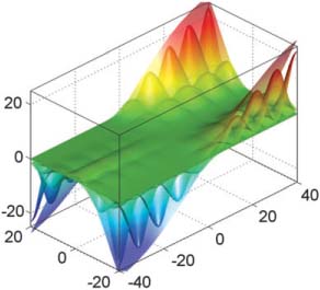
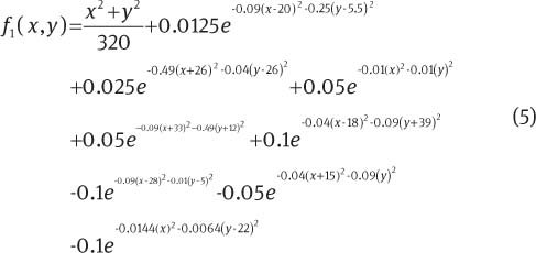
In this section, we describe an application of the hybrid RBF and local ϕ-polynomials method, specifically Zernike polynomials, for the description of an extremely asymmetric surface. The surface is chosen to be a stressing example of departure from rotational symmetry. It does, however, represent a descriptive case for spatial frequency. The surface is an F/1 parabola over an 80 mm×80mm rectangular domain with several 12.5 μm–100 μm isotropic and anisotropic bumps distributed over the aperture. An analytical description of the surface is given in Eq. (5). In Figure 6we show the F/1 parabola (with several bumps over the rectangular aperture) to mainly show the overall sag of the surface.

F/1 Parabola where 12.5 μm–100 μm bumps may be visualized in Figure 7.
In Figure 7we isolate the bumps on the surface. There are radially symmetric and anisotropic bumps of several heights in the range between 12.5 μm and 100 μm. We have sampled the representative freeform surface with 600×600 uniform samples, and evaluated the overall fit with 120×120 uniform points. The shape parameter for the weight function, which is a Wendland’s C2 function, is 1.25 mm-1. As for the local approximations, we have made use of 36 FRINGE Zernike polynomials. We have decomposed the domain with 100×100 overlapping circular subapertures. The radius of each subaperture is 800 μm. In Figure 8we show the decomposition of the full aperture between -2mm and 2mm with 800 μm circular subapertures. We can observe the uniform distribution of samples (blue points) along with a grid of uniform evaluation points (red points). As shown in our earlier work, there is actually no difference in surface approximation performance of ϕ-polynomials with uniform or clustered samples when the number of ϕ-polynomials is low [21], such as in this case, 36, we make use of a uniform grid of samples across the overall aperture.

The 12.5 μm–100 μm isotropic and anisotropic bumps configuration on F/1 parabola over an 80 mm×80mm square aperture.

Decomposition of the aperture of an F/1 parabola with 800 μm circular subapertures along with uniformly distributed sample points, shown only for a -2mm to 2mm cross-section.
Although the number of the FRINGE Zernike polynomials used in local subapertures is only 36, we have obtained excellent approximation errors on the orders of the subnanometer.
In Figure 9we show the peak-to-valley (PV) approximation error profile for the F/1 parabola with several bumps. Results show that the approximation PV errors are less than or equal to around 0.3 nm. There are no edge-related oscillation errors even with uniform sampling. Nonetheless, errors concentrate around the 25 μm and 50 μm anisotropic bumps whose slopes are the largest [see lines 2 and 3 in Eq. (5)]. The overall root mean square error for this description is 0.01 nm. Given the oscillatory nature of the errors, while at subnanometer scale, smoothing of the computed surface would further decrease their magnitude.

Approximation error profile for an F/1 parabola with several bumps showing the maximum PV errors on the orders of the subnanometer with only 36 FRINGE Zernike polynomials across an 80 mm×80mm aperture.
We have carried out the F/1 parabola with bumps test with 25, 36, and 64 Zernike polynomials in local subaperture surface approximations. We have recorded the radius of the subaperture along with the number of subapertures in order to reach subnanometer PV errors. The shape parameter for Wendland’s CSRBFs for each experiment is the inverse of the radius of the subapertures listed in column 2 of Table 1.Table 1 summarizes the results. As the number of local Zernike polynomials in the local approximation increases from 25 to 64, the radius of the subaperture increases from 610 μm to 1.33 mm. At the same time, the number of subapertures decreases from 130×130 to 60×60. The more Zernike polynomials that are added into the approximation set, the more capable the method becomes in terms of locally describing a freeform surface, and thus we can increase the radius of the subaperture. This trade-off is well captured in Table 1.
Subnanometer PV errors with a small set of Zernike polynomials (4th column) or Gaussian RBFs (5th column).
| Cell count | Cell radius (mm) | Number of local basis elements | PV error Zernike (nm) | PV error Gaussian (nm) |
|---|---|---|---|---|
| 60×60 | 1.33 | 64 | 0.2 | 1.01 |
| 100×100 | 0.8 | 36 | 0.31 | 2.29 |
| 130×130 | 0.61 | 25 | 0.78 | 3.59 |
In Table 1, we also compare a simple version of the Gaussian RBFs as local surface approximants to that using a small number of Zernike polynomials needed to represent the surface using in both cases the hybrid method. In this investigation, we included a shape optimization, where ε was varied from 0.01mm-1 to 10mm-1 for Gaussians over each subaperture. Every other parameter, i.e., number of samples and their uniform distribution, was kept the same. As we varied the number of Gaussians, results show that although local Gaussians within subapertures provide accuracies around nanometers, Zernike polynomials provide accuracies on the orders of subnanometers. However, Gaussian RBF implementation may still be improved with different sampling and basis center distributions. In [19], different grid types were applied for approximation with Gaussian RBFs and results concluded that residual errors are comparable to polynomial approximation counterparts. Also, in [28], the authors compared different edge remedies for improving the errors of RBF approximations, including clustering the sample points towards the boundary and two possible Not-a-Knot implementations. Without incurring any additional computational cost, methods mentioned in [28] for improving Gaussian RBF approximation errors may be applied within each subdomain.
Instead of using a fixed uniform grid of samples and uniform decomposition of the overall aperture into subapertures, an adaptive approach may be used instead for the domain decomposition and sampling steps. For example, Driscoll and Heryudono present an adaptive refinement method based upon residual subsampling [23]. This adaptive method clusters the samples and the subapertures around the steep regions, whereas it coarsens the samples and subapertures around the large smooth areas. By clustering the samples towards the steep gradients and locally increasing the density of subapertures around the steep regions, more accuracy can be achieved and significant benefits in terms of cost, especially for local RBF approximations, can be gained, where a local shape optimization can be carried out based on the density of the RBF centers.
Another possible improvement for the Gaussian RBF approximations is to use an approach that is presented in [29] that allows selecting sample and center locations along with an optimum shape parameter for each and every RBF basis. This method has shown significant advantages compared with orthogonal polynomials in 1D such as the reduction in the number of basis elements as compared with Chebyshev polynomials [29].
As an additional experiment, we have carried out an F/1 parabola with bumps with 16, 25, 36, and 64 Zernike polynomials in local subapertures while recording the radius of the subapertures and their total number in order to reach 10nm PV accuracy. Results reported in Table 2 show that as few as 16 ϕ-polynomials can describe this surface with 10nm PV errors. As the number of ϕ-polynomials decreases from 64 to 16, the radius of the subapertures decreases from 2.29mm to 670 μm, whereas the number of subapertures increases from 35×35 to 120×120 to reach 10nm PV errors.
Illustration of 10nm PV errors with a small set of Zernike polynomials.
| Cell count | Cell radius (mm) | Number of local basis elements | PV error (nm) |
|---|---|---|---|
| 35×35 | 2.29 | 64 | 10.06 |
| 57×57 | 1.40 | 36 | 6.07 |
| 75×75 | 1.07 | 25 | 9.35 |
| 120×120 | 0.67 | 16 | 8.41 |
In summary, the numerical experiments quantify that a small set of FRINGE Zernike polynomials, 25, are able to describe the overall surface within a non-circular aperture with the hybrid RBF local Zernike method within subnanometer accuracies. The analysis further shows that fewer polynomials are needed if the requirement on accuracy is loosened.
5 Conclusion
As the optics manufacturing industry is forging ahead in the advancement of their methods, freeform optical elements are going to be key components of optical systems in the near future. In this paper, we describe a fast, efficient hybrid method combining local approximants (i.e., RBFs or ϕ-polynomials) and RBF global approximants. With this method, we are able to describe a freeform surface with, for example, only 25 FRINGE Zernike polynomials within subnanometer accuracy. With a simple RBF local approximant and 25–64 basis functions, nanometer-level accuracy was achieved. Because of its local nature and the ability to carry the local accuracies over to the overall surface description, this hybrid method reduces the number of basis functions required to describe a freeform surface. The method is highly efficient mainly because of three inherent properties. First, the method makes use of Wendland’s CSRBFs that are known to best handle large datasets; also they result in band diagonal approximation matrices that are simple to manipulate in algebraic systems. Second, to find the local samples and evaluation points, we make use of kd-trees for containment queries, which reduces computational complexity to an O[log(N)] process. A third reason for efficiency is the fact that the number of local basis functions is kept to a minimum, which results in small approximation matrices. In the case of ϕ-polynomials, using a small number of them allowed us to use uniform sampling without an approximation performance penalty. Reducing the number of Zernike polynomials to a minimum is also important because it facilitates understanding of the local optical properties of the surface for optical designers while providing computational advantages. We also note that there is no inherent limit in terms of the number of local ϕ-polynomials that may be used in the method; in order to achieve better accuracies than subnanometers, that is, machine precision, high-order polynomials may also be used within the local subapertures. Finally, the Q-polynomials or other ϕ-polynomials may substitute within local subapertures the Zernike polynomials. However, a crucial step working with Q-polynomials is to accurately compute the curvature of the best-fit sphere, which requires a mean sag over the perimeter of the local subaperture as a targeted step into the hybrid algorithm.
About the authors

Ilhan Kaya is a PhD student in the Department of Electrical Engineering and Computer Science at University of Central Florida, supervised by Prof. Jannick Rolland. Ilhan Kaya graduated from Electrical and Electronics Engineering at Bilkent University before he received a Master’s of Science Degree in Computer Engineering at Bogaziçi University in Turkey. Currently, Ilhan Kaya’s research interests are in computational modeling, simulation, and visualization with a focus on freeform optics.

Jannick Rolland is the Brian J. Thompson Professor of Optical Engineering at the Institute of Optics at the University of Rochester and the director of the R.E. Hopkins Center for Optical Design and Engineering, the planned NSF Center for Freeform Optics (CeFO), and the ODALab (www.odalab-spectrum.org). Professor Rolland holds appointments in the Department of Biomedical Engineering and in the Center for Visual Science. Jannick Rolland received an Optical Engineering Diploma from the Institut D’Optique, France, and a PhD in Optical Science from the College of Optical Sciences at the University of Arizona. Professor Rolland is a NYSTAR Fellow and a Fellow of OSA and SPIE. Professor Rolland’s interest lies in freeform optics and optical instrumentation innovation across a broad range of applications, with a key focus on metrology, 3D biomedical imaging, and head-worn displays for augmented reality. Professor Roland is a Director at Large on the OSA Board of Directors.
This work was supported by the National Science Foundation GOALI grant ECCS-1002179, the II-VI Foundation, and the NYSTAR Foundation C050070. We thank Kevin Thompson for stimulating discussions about this work.
References
[1] O. Cakmakci and J. P. Rolland, J. Disp. Technol. 2, 199–216 (2006).10.1109/JDT.2006.879846Search in Google Scholar
[2] J. P. Rolland, K. P. Thompson, H. Urey and M. Thomas, in ‘Handbook of Visual Display Technology’, Ed. by J. Chen, W. Cranton and M. Fihn (Springer, Bristol, UK, 2012) pp. 2145–2170.10.1007/978-3-540-79567-4_134Search in Google Scholar
[3] J. C. Minano, P. Benitez and A. Santamaria, Opt. Rev. 16, 99–102 (2009).Search in Google Scholar
[4] K. Fuerschbach, J. P. Rolland and K. P. Thompson, Opt. Express 19, 21919–21928 (2011).10.1364/OE.19.021919Search in Google Scholar PubMed
[5] M. Born and E. Wolf, in ‘Principles of Optics’ (Cambridge University Press, Cambridge, 1999).Search in Google Scholar
[6] G. W. Forbes, Opt. Express 15, 5218–5226 (2007).10.1364/OE.15.005218Search in Google Scholar PubMed
[7] G. Fasshauer, in ‘Meshfree Approximation Methods with MATLAB’ (World Scientific Publishing, Singapore, 2007).10.1142/6437Search in Google Scholar
[8] O. Cakmakci, B. Moore, H. Foroosh and J. P. Rolland, Opt. Express 16, 1583–1589 (2008).10.1364/OE.16.001583Search in Google Scholar
[9] G. W. Forbes, Opt. Express 18, 13851–13862 (2010).10.1364/OE.18.013851Search in Google Scholar PubMed
[10] J. J. Koenderink, in ‘Solid Shape’ (The MIT Press, Cambridge, 1990).Search in Google Scholar
[11] F. Roddier, Appl. Optics 27, 1223–1225 (1988).Search in Google Scholar
[12] P. E. Glenn, Proc. SPIE1333, 230–238 (1990).Search in Google Scholar
[13] W. Zou and J. P. Rolland, US Patent 7,390,999 (2008).Search in Google Scholar
[14] W. Zou, K. P. Thompson and J. P. Rolland, JOSA A 25, 2331–2337 (2008).10.1364/JOSAA.25.002331Search in Google Scholar
[15] Y.-M. Liu, G. Lawrence and C. Koliopoulos, Appl. Optics 27, 4504–4513 (1988).Search in Google Scholar
[16] E. Abbe, US Patent 697,959 (April, 1902).Search in Google Scholar
[17] G. W. Forbes, Opt. Express 19, 9923–9941 (2011).10.1364/OE.19.009923Search in Google Scholar PubMed
[18] R. W. Gray, C. Dunn, K. P. Thompson and J. P. Rolland, Opt. Express 20, 16436–16449 (2012).10.1364/OE.20.016436Search in Google Scholar
[19] J. P. Boyd and F. Yu, J. Comput. Phys. 230, 1408–1438 (2011).Search in Google Scholar
[20] I. Kaya, K. P. Thompson and J. P. Rolland, Opt. Express 19, 26962–26974 (2011).10.1364/OE.19.026962Search in Google Scholar
[21] I. Kaya, K. P. Thompson and J. P. Rolland, Opt. Express 20, 22684–22691 (2012).Search in Google Scholar
[22] G. W. Forbes, Opt. Express 20, 2483–2499 (2012).10.1364/OE.20.002483Search in Google Scholar
[23] T. A. Driscoll and A. R. H. Heryudono, Comp. Math. Appl. 53, 927–939 (2007).Search in Google Scholar
[24] T. A. Driscoll and B. Fornberg, Comput. Math. Appl. 43, 413–422 (2002).Search in Google Scholar
[25] B. Fornberg, E. Larsson and N. Flyer, SIAM J. Sci. Comput. 33, 869–892 (2011).10.1137/09076756XSearch in Google Scholar
[26] G. Fasshauer and M. McCourt, SIAM J. Sci. Comput. 34, A737–A762 (2012).10.1137/110824784Search in Google Scholar
[27] M. Abramowitz and I. Stegun, in ‘Handbook of Mathematical Functions’ (Dover, New York, 1972).Search in Google Scholar
[28] B. Fornberg, T. A. Driscoll, G. Wright and R. Charles, Comp. Math. Appl. 43, 473–490 (2002).10.1016/S0898-1221(01)00299-1Search in Google Scholar
[29] B. Fornberg and J. Zuev, Comp. Math. Appl. 54, 379–398 (2007).Search in Google Scholar
©2013 by THOSS Media & De Gruyter Berlin Boston
Articles in the same Issue
- Masthead
- Masthead
- Publisher’s Note
- Starting an optics journal in troubled times
- Community
- News from The European Optical Society
- Conference Notes
- Conference Calendar
- Topical Issue: Optical Design
- Editorial
- Editorial
- Tutorials
- The modern miniature camera objective: an evolutionary design path from the landscape lens
- Lens design: optimization with Global Explorer
- Q and A tutorial on optical design
- The importance of induced aberrations in the correction of secondary color
- Review Article
- Lens designs with extreme image quality features
- Research Articles
- Desensitization of axially asymmetric optical systems
- Extrinsic aberrations in optical imaging systems
- Hybrid RBF and local ϕ-polynomial freeform surfaces
- The astigmatic aberration field in active primary mirror astronomical telescopes
- Optical design with orthogonal representations of rotationally symmetric and freeform aspheres
- A new prime-focus corrector for paraboloid mirrors