Home Long-time asymptotic behavior for the Hermitian symmetric space derivative nonlinear Schrödinger equation
Article Open Access

Long-time asymptotic behavior for the Hermitian symmetric space derivative nonlinear Schrödinger equation

  • Mingming Chen , Xianguo Geng EMAIL logo and Huan Liu
Published/Copyright: June 11, 2024

Abstract

Resorting to the spectral analysis of the 4 × 4 matrix spectral problem, we construct a 4 × 4 matrix Riemann–Hilbert problem to solve the initial value problem for the Hermitian symmetric space derivative nonlinear Schrödinger equation. The nonlinear steepest decent method is extended to study the 4 × 4 matrix Riemann–Hilbert problem, from which the various Deift–Zhou contour deformations and the motivation behind them are given. Through some proper transformations between the corresponding Riemann–Hilbert problems, the basic Riemann–Hilbert problem is reduced to a model Riemann–Hilbert problem, by which the long-time asymptotic behavior to the solution of the initial value problem for the Hermitian symmetric space derivative nonlinear Schrödinger equation is obtained with the help of the asymptotic expansion of the parabolic cylinder function and strict error estimates.

MSC 2020: 35Q55; 35B40; 35Q15

1 Introduction

The derivative nonlinear Schrödinger (DNLS) equation

(1.1) i q t + q x x + 2 i ( | q | 2 q ) x = 0 ,

is one of the basic models in integrable systems. This equation describes the propagation of nonlinear pulses in nonlinear fiber optics [1], [2] and arises as a model for Alfvén waves propagating parallel to the ambient magnetic field in the plasma physics [3]. Equation (1.1) has also several interesting properties in mathematics. In Ref. [4], Kaup and Newell studied the DNLS Equation (1.1) by means of inverse scattering transformation and derived its infinity of conservation laws. N-soliton solution of the DNLS Equation (1.1) was obtained by resorting to the Darboux transformation [5]. The unique global existence of solutions for the DNLS Equation (1.1) was proved under an explicit smallness condition of the initial data in Sobolev spaces and the Schwartz class [6]. Explicit quasi-periodic solutions for the coupled DNLS hierarchy were given with the help of algebraic-geometric method [7]. The long-time asymptotics of the solution of the initial value problem and the initial-boundary value problem for the DNLS Equation (1.1) are studied in the basis of the nonlinear steepest descent analysis of the associated Riemann–Hilbert problem [8], [9], [10]. Moreover, the integrability and exact solutions for multi-coupled versions of the nonlinear Schrödinger equation and derivative nonlinear Schrödinger equation have also been discussed extensively in Ref. [11] by resorting to the Darboux transformation, Riccati equation, and Baker-Akhiezer function [12], [13], [14], [15], [16], [17], [18], [19], [20].

The nonlinear steepest descent method was first introduced by Deift and Zhou in Ref. [21]. This method provides a powerful tool to reduce the original 2 × 2 matrix Riemann–Hilbert problem to a canonical model Riemann–Hilbert problem whose solution can be precisely expressed in terms of parabolic cylinder functions, by which the long-time asymptotics for the initial value problems to a lot of integrable nonlinear evolution equations associated with 2 × 2 matrix spectral problems was obtained, (see e.g. [8], [9], [10], [21], [22], [23], [24], [25], [26], [27], [28], [29], [30]). However, there is little literature on the long-time asymptotic behavior of solutions for integrable nonlinear evolution equations associated with 3 × 3 matrix spectral problems. Usually, it is difficult and complicated for the 3 × 3 case. For 2 × 2 and 3 × 3 cases, the former corresponds to a scalar Riemann–Hilbert problem, while the latter corresponds to a matrix Riemann–Hilbert problem. In general, the solution of the matrix Riemann–Hilbert problem can not be given in explicit form, but the scalar Riemann–Hilbert problem can be solved by the Plemelj formula. Recently, the nonlinear steepest descent method was successfully generalized to study the long-time asymptotics of the initial value problems for the nonlinear evolution equations related to higher-order matrix spectral problems, for example, the coupled nonlinear Schrödinger equation, the Sasa-Satuma equation, the Degasperis-Procesi equation and so on [31], [32], [33], [34], [35], [36].

In this paper, the nonlinear steepest decent method is extended to study the long-time asymptotic behavior of solutions for the initial value problem of the Hermitian symmetric space derivative nonlinear Schrödinger (HSS-DNLS) equation associated with 4 × 4 matrix spectral problem

(1.2) i q 1 t + q 1 x x + i | q 1 | 2 + 2 | q 0 | 2 q 1 + q 0 2 q 1 * x = 0 , i q 0 t + q 0 x x + i | q 1 | 2 + | q 0 | 2 + | q 1 | 2 q 0 + q 1 q 0 * q 1 x = 0 , i q 1 t + q 1 x x + i 2 | q 0 | 2 + | q 1 | 2 q 1 + q 0 2 q 1 * x = 0 ,

with the initial data

(1.3) q j ( x , 0 ) = q j , 0 ( x ) , j ± 1,0 ,

where the asterisk represents the complex conjugate, potentials q ±1 and q 0 are three complex-valued functions with two real independent variables x and t. The initial data q j,0(x) lie in the Schwartz space S ( R ) = f ( x ) C ( R ) : sup x R | x α β f ( x ) | < , α , β N . And q j,0(x) are assumed to be generic so that the matrices s 12(λ) and s 22(λ) defined in (2.24) are invertible in D (Figure 1). If we set q 1 = q 0 = −q −1, Equation (1.2) can be reduced to the DNLS Equation (1.1). In addition, the dynamical behaviors of all types of solutions of the HSS-DNLS Equation (1.2) are discussed in detail via the Darboux transformation [37].

Figure 1: 
The contour 


Γ

̂


$\hat{{\Gamma}}$


 and the domains D
± in the complex λ-plane.
Figure 1:

The contour Γ ̂ and the domains D ± in the complex λ-plane.

It is very difficult for us to carry out the spectrum analysis and the inverse scattering transformation because the associated spectral problem is a high-order matrix spectral problem, the 4 × 4 matrix spectral problem. The Hermitian symmetric space derivative nonlinear Schrödinger equation corresponds to the 4 × 4 matrix Riemannt–Hilbert problem, which is reduced to two 2 × 2 matrix Riemannt–Hilbert problems. However, the unsolvability of them is a challenge for us. The main result of this paper is as follows:

Theorem 1.1.

Let q j (x, t) be the solution of the initial value problem for the HSS-DNLS Equation (1.2) with the initial data q j , 0 ( x ) S ( R ) . Then, for x < 0 and x 4 t > C , as t → ∞, the leading asymptotics of q j (x, t) has the form

(1.4) q 1 q 0 q 0 q 1 = 1 16 π t λ 0 2 2 i ν ν Γ ( i ν ) e 3 π i 4 + π ν 2 δ A 0 2 + δ B 0 2 W 0 T γ ( λ 0 ) W 0 + O log t t λ 0 2 ,

where C R is a fixed constant and C > 0, the error term is uniform with respect to x, Γ(⋅) is the Gamma function, the matrix valued function γ(λ) is defined in (2.33), and

δ A 0 = 16 t λ 0 4 i ν 2 exp 2 i t λ 0 4 + χ + ( λ 0 ) + χ ( λ 0 ) + χ ̂ + ( λ 0 ) + χ ̂ ( λ 0 ) ,

δ B 0 = 16 t λ 0 4 i ν 2 exp 2 i t λ 0 4 + χ + ( λ 0 ) + χ ( λ 0 ) + χ ̂ + ( λ 0 ) + χ ̂ ( λ 0 ) , δ ̃ A 0 ( λ ) = ( 16 t λ 4 ) i ν 2 exp 2 i t λ 4 + χ + ( λ ) + χ ( λ ) + χ ̂ + ( λ ) + χ ̂ ( λ ) , δ ̃ B 0 ( λ ) = ( 16 t λ 4 ) i ν 2 exp 2 i t λ 4 + χ + ( λ ) + χ ( λ ) + χ ̂ + ( λ ) + χ ̂ ( λ ) , λ 0 = x 4 t , ν = 1 2 π log ( 1 + | γ ( λ 0 ) | 2 + | det γ ( λ 0 ) | 2 ) , ν ̃ ( λ ) = 1 2 π log ( 1 + | γ ( λ ) | 2 + | det γ ( λ ) | 2 ) , W 0 = I 2 × 2 + i 2 λ 0 2 + δ ̃ A 0 ( s ) δ ̃ B 0 ( s ) 2 + δ ̃ B 0 ( s ) δ ̃ A 0 ( s ) 2 ν ̃ ( s ) s ( 1 e 2 π ν ̃ ( s ) ) γ ( s ) γ ( s ) d s , χ ± ( λ l ) = 1 2 π i 0 ± λ 0 log 1 + | γ ( ξ ) | 2 + | det γ ( ξ ) | 2 1 + | γ ( λ 0 ) | 2 + | det γ ( λ 0 ) | 2 d ξ ξ λ l , χ ̂ ± ( λ l ) = 1 2 π i ± 0 log 1 | γ ( i ξ ) | 2 + | det γ ( i ξ ) | 2 d log ( i ξ λ l ) , l { 1,2 } , λ 1 = λ 0 , λ 2 = λ 0 .

Remark 1.

For convenience, we introduce the basic notations: (1) For any matrix A = (a ij ) (may not be square), the norm of matrix A is defined as | A | i , j | a i j | 2 1 2 = ( t r A A ) 1 2 , where † denotes the Hermite conjugate; (2) We say A is in L p ( Ω ) for some contour Ω C if each of the entries a i j L p ( Ω ) , then we define A ( ) L p | A ( ) | L p ; (3) If A is a 4 × 4 matrix, it can be written as the block form

(1.5) A = A 11 A 12 A 21 A 22 ,

where A 11, A 12, A 21 and A 22 are all 2 × 2 matrices; (4) For two quantities A and B, AB if there exists a constant C > 0 such that |A| ≤ CB. In particular, if C depends on the parameter α, then we say that A α B.

The outline of this paper is as follows. In Section 2, based on the spectral analysis and inverse scattering transformation, we show how to transform the solution of the initial value problem for the HSS-DNLS equation into the solution of a 4 × 4 matrix Riemann–Hilbert problem. In Section 3, by using the nonlinear steepest descent method, the original 4 × 4 matrix Riemann–Hilbert problem can be reduced to a model Riemann–Hilbert problem whose solution can be expressed in terms of the parabolic cylinder functions. We finally obtain the long-time asymptotics of the initial value problem for the HSS-DNLS equation. The detailed proof of Theorems 3.1, 3.4, and 3.5 is given in Appendix A.

2 Riemann–Hilbert problem

2.1 Spectral analysis

The HSS-DNLS Equation (1.2) is the compatibility condition of the Lax pair equations

(2.1) ψ x = i λ 2 σ 4 + U ̃ ψ ,

(2.2) ψ t = 2 i λ 4 σ 4 + V ̃ ψ ,

where λ C is the spectral parameter, ψ = ψ(λ; x, t) is a 4 × 4 matrix valued function,

U ̃ = 0 2 × 2 λ Q λ Q 0 2 × 2 , V ̃ = V ̃ 11 V ̃ 12 V ̃ 21 V ̃ 22 , Q = q 1 q 0 q 0 q 1 , σ 4 = I 2 × 2 0 2 × 2 0 2 × 2 I 2 × 2 .

V ̃ 11 = i λ 2 Q Q , V ̃ 12 = 2 λ 3 Q + i λ Q x + i Q Q Q , V ̃ 21 = 2 λ 3 Q + i λ Q x i Q Q Q , V ̃ 22 = i λ 2 Q Q .

We introduce the transformation

(2.3) ϕ ( λ ; x , t ) = ψ ( λ ; x , t ) e i λ 2 σ 4 x 2 i λ 4 σ 4 t ,

where e σ 4 = diag e 1 , e 1 , e,e . From (2.1) and (2.2), we can deduce the Lax pair of ϕ(λ; x, t)

(2.4) ϕ x = i λ 2 [ σ 4 , ϕ ] + U ̃ ϕ ,

(2.5) ϕ t = 2 i λ 4 [ σ 4 , ϕ ] + V ̃ ϕ ,

which can be written in differential form

(2.6) d ( e i λ 2 x σ ̂ 4 2 i λ 4 t σ ̂ 4 ϕ ( λ ; x , t ) ) = e i λ 2 x σ ̂ 4 2 i λ 4 t σ ̂ 4 ( U ̃ ϕ ( λ ; x , t ) d x + V ̃ ϕ ( λ ; x , t ) d t ) ,

where e σ ̂ 4 acts on a 4 × 4 matrix A is that e σ ̂ 4 A = e σ 4 A e σ 4 .

In order to obtain the original Riemann–Hilbert problem related to the initial value problem for the HSS-DNLS Equation (1.2), it is necessary that solutions of the spectral problem approach the identity matrix I 4×4. Note that the solutions of Equation (2.6) do not exhibit this property. Hence, our next step is to transform the Equation (2.6) for ϕ(λ; x, t) into an equation with the desired asymptotic behavior. For this purpose, we define

(2.7) Y ( x , t ) = W * ( x , t ) 0 2 × 2 0 2 × 2 W ( x , t ) ,

where W(x, t) is a 2 × 2 matrix valued function and satisfies

(2.8) W x = i 2 Q Q W , W t = 3 i 4 Q Q Q Q + 1 2 Q x Q 1 2 Q Q x W

with the asymptotic condition W(x, t) → I 2×2 as x → −∞, t = 0. It is easy to see that W −1(x, t) = W (x, t), and W(x, t) satisfies the integral equation

(2.9) W ( x , t ) = I 2 × 2 + ( , 0 ) ( x , t ) i 2 Q Q W ( x , t ) d x + 3 i 4 Q Q Q Q + 1 2 Q x Q 1 2 Q Q x W ( x , t ) d t .

Again introducing a transformation

(2.10) μ ( λ ; x , t ) = Y 1 ( x , t ) ϕ ( λ ; x , t ) ,

we can deduce by (2.4) and (2.5) that the Lax pair of μ(λ; x, t)

(2.11) μ x = i λ 2 [ σ 4 , μ ] + U μ ,

(2.12) μ t = 2 i λ 4 [ σ 4 , μ ] + V μ ,

where

(2.13) U = Y 1 U ̃ Y Y 1 Y x , V = Y 1 V ̃ Y Y 1 Y t .

The Lax pair of μ(λ; x, t) can be written in differential form

(2.14) d ( e i λ 2 x σ ̂ 4 2 i λ 4 t σ ̂ 4 μ ( λ ; x , t ) ) = e i λ 2 x σ ̂ 4 2 i λ 4 t σ ̂ 4 ( U μ ( λ ; x , t ) d x + V μ ( λ ; x , t ) d t ) .

From (2.13), the 4 × 4 matrix U has the block form

(2.15) U = i 2 W T Q Q W * λ W T Q W λ W 1 Q W * i 2 W 1 Q Q W .

We define two matrix Jost solutions μ ± = μ ±(λ; x, t) of Equation (2.11) by the Volterra integral equations

(2.16) μ ± ( λ ; x , t ) = I 4 × 4 + ± x e i λ 2 σ ̂ 4 ( x ξ ) U ( ξ , t ) μ ± ( λ ; ξ , t ) d ξ ,

with the asymptotic conditions

(2.17) μ ± I 4 × 4 , x ± .

2.2 Analyticity and the symmetry relations

Let

(2.18) μ + = ( μ + L , μ + R ) , μ = ( μ L , μ R ) ,

where μ ±L and μ ±R denote the first two columns and latter two columns of μ ±. The existence and uniqueness of Jost solutions μ ± for integral Equation (2.16) can be proved according to the standard procedures [38]. A direct observation shows by using the integral Equations (2.16) that μ L and μ +R are continuous in D + Γ ̂ and analytic in D +, μ +L and μ R are continuous in D Γ ̂ and analytic in D (see Figure 1), where

Γ ̂ = { λ : I m ( λ 2 ) = 0 } , D + = { λ C | arg λ ( 0 , π / 2 ) ( π , π / 2 ) } , D = { λ C | arg λ ( π / 2 , π ) ( π / 2,0 ) } .

From (2.3) and (2.10), we know that Y μ ± e i λ 2 σ 4 x + 2 i λ 4 σ 4 t are two solutions of Lax Equations (2.1) and (2.2), they’re linearly dependent so that there’s a scattering matrix s(λ) that makes

(2.19) μ e i λ 2 σ 4 x + 2 i λ 4 σ 4 t = μ + e i λ 2 σ 4 x + 2 i λ 4 σ 4 t s ( λ ) , λ Γ ̂ .

Note that matrix U in (2.15) is traceless, one can infer that det μ ± are independent of the variable x. Furthermore, by (2.16), we calculate det μ ± = 1 at x = ±∞, hence

(2.20) det μ ± = 1 , λ Γ ̂ .

Combining with (2.19), we find that det s(λ) = 1. The matrix U in (2.15) satisfies the following two symmetry relations

(2.21) U ( λ * ) = U ( λ ) , σ 4 U ( λ ) σ 4 = U ( λ ) .

It follows from (2.11) that

(2.22) μ ± ( λ * ) = μ ± 1 ( λ ) , σ 4 μ ± ( λ ) σ 4 = μ ± ( λ ) .

Therefore, we obtain by (2.19) that

(2.23) s ( λ * ) = s 1 ( λ ) , σ 4 s ( λ ) σ 4 = s ( λ ) .

The 4 × 4 scattering matrix s(λ) can be rewritten in a block form

(2.24) s ( λ ) = s 11 ( λ ) s 12 ( λ ) s 21 ( λ ) s 22 ( λ ) .

We suppose that s 12(λ) and s 22(λ) are invertible in the domain D . By (2.23), It is easy to verify that

(2.25) s 11 ( λ * ) = s 11 ( λ ) s 12 ( λ ) s 22 1 ( λ ) s 21 ( λ ) 1 , s 12 ( λ ) = s 12 ( λ ) ,

(2.26) s 21 ( λ * ) = s 21 ( λ ) s 22 ( λ ) s 12 1 ( λ ) s 11 ( λ ) 1 , s 22 ( λ ) = s 22 ( λ ) .

Taking t = 0 and x → +∞ in (2.19), we can infer that scattering matrix s(λ) satisfies the integral equation

(2.27) s ( λ ) = lim x + e i λ 2 σ ̂ 4 x μ ( λ ; x , 0 ) = I 4 × 4 + + e i λ 2 σ ̂ 4 ξ U ( ξ , 0 ) μ ( λ ; ξ , 0 ) d ξ ,

which implies

(2.28) s 12 ( λ ) = + e 2 i λ 2 ξ i 2 W T ( ξ , 0 ) Q ( ξ , 0 ) Q ( ξ , 0 ) W * ( ξ , 0 ) μ 12 ( λ ; ξ , 0 ) + λ W T ( ξ , 0 ) Q ( ξ , 0 ) W ( ξ , 0 ) μ 22 ( λ ; ξ , 0 ) d ξ ,

(2.29) s 22 ( λ ) = I 2 × 2 + λ W 1 ( ξ , 0 ) Q ( ξ , 0 ) W * ( ξ , 0 ) μ 12 ( λ ; ξ , 0 ) + i 2 W 1 ( ξ , 0 ) Q ( ξ , 0 ) Q ( ξ , 0 ) W ( ξ , 0 ) μ 22 ( λ ; ξ , 0 ) d ξ .

2.3 The Riemann–Hilbert problem

Define

(2.30) M ( λ ; x , t ) = μ L s 11 1 ( λ ) , μ + R , λ D + , μ + L , μ R s 22 1 ( λ ) , λ D .

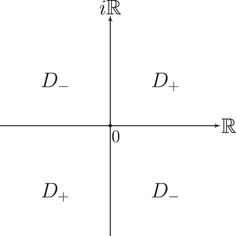
In fact, by using formula (2.19) and definition (2.30), we find that the matrix M(λ; x, t) is analytic in λ C \ Γ ̂ and is the unique solution of the Riemann–Hilbert problem on Γ ̂ (see Figure 2)

(2.31) M + ( λ ; x , t ) = M ( λ ; x , t ) J ( λ ; x , t ) , λ Γ ̂ , M ( λ ; x , t ) I 4 × 4 , λ ,

where the left and the right boundary values along the oriented contour on Γ ̂ are denoted by M +(λ; x, t) and M (λ; x, t), respectively,

(2.32) J ( λ ; x , t ) = I 2 × 2 + γ ( λ ) γ ( λ * ) e 2 i t θ γ ( λ ) e 2 i t θ γ ( λ * ) I 2 × 2 ,

(2.33) θ ( λ ; x , t ) = x t λ 2 + 2 λ 4 , γ ( λ ) = s 12 ( λ ) s 22 1 ( λ ) .

Figure 2: 
The oriented contour on 


Γ

̂


$\hat{{\Gamma}}$


.
Figure 2:

The oriented contour on Γ ̂ .

The 2 × 2 matrix valued function γ(λ) is the reflection coefficient corresponding to the initial data q j,0(x). It lies in the Schwartz space S ( R ) and satisfies

(2.34) sup λ Γ ̂ | γ ( λ ) | < 1 , γ ( λ ) = γ ( λ ) .

It is obvious that the jump matrix J(λ; x, t) is positive definite, the existence and uniqueness of the solution of the Riemann–Hilbert problem (2.31) can be guaranteed by the Vanishing Lemma [39].

Theorem 2.1.

The solution of the initial value problem for the HSS-DNLS Equation (1.2) can be expressed as

(2.35) Q ( x , t ) = q 1 ( x , t ) q 0 ( x , t ) q 0 ( x , t ) q 1 ( x , t ) = W * Q ̃ W 1 ,

where

(2.36) Q ̃ ( x , t ) 2 i lim λ ( λ M ( λ ; x , t ) ) 12 .

Proof.

M(λ; x, t) admits the asymptotic expansion

(2.37) M ( λ ; x , t ) = I 4 × 4 + M 1 ( x , t ) λ + M 2 ( x , t ) λ 2 + O ( λ 3 ) , λ .

Substituting (2.37) into (2.11), we obtain (2.35) and (2.36). □

3 Long-time asymptotic behavior

In this section, by using the nonlinear steepest descent method, the original Riemann–Hilbert problem (2.31) can be reduced to a model Riemann–Hilbert problem with constant coefficients after several appropriate transformations. We then obtain the long-time asymptotics of the HSS-DNLS Equation (1.2) with the leading term.

3.1 Transformation of the Riemann–Hilbert problem

The key step of the method is to transform the original Riemann–Hilbert problem according to the signature table for the phase function θ in jump matrix J defined in (2.32). It follows that there are three stationary points ± x 4 t and 0 at θ λ = 0 . For convenience, let’s define

(3.1) λ 0 = x 4 t , λ 0 = x 4 t .

To have a better understanding, we denote λ by λ = λ R + I , where λ R , λ I R . Then

(3.2) R e ( i θ ) = 8 λ R λ I λ R 2 + λ I 2 + λ 0 2 .

Therefore, the signature table of the real part of can be depicted in Figure 3.

Figure 3: 
The signature table for Re(iθ) in the complex λ-plane.
Figure 3:

The signature table for Re() in the complex λ-plane.

Now, we introduce two 2 × 2 matrix valued functions δ 1(λ) and δ 2(λ), which satisfy the Riemann–Hilbert problems, respectively

(3.3) δ 1 + ( λ ) = δ 1 ( λ ) T 1 ( λ ) , λ ( λ 0 , λ 0 ) ( i , + i ) , δ 1 + ( λ ) = δ 1 ( λ ) , λ ( , λ 0 ) ( λ 0 , + ) , δ 1 ( λ ) I 2 × 2 , λ .

(3.4) δ 2 + ( λ ) = T 2 ( λ ) δ 2 ( λ ) , λ ( λ 0 , λ 0 ) ( i , + i ) , δ 2 + ( λ ) = δ 2 ( λ ) , λ ( , λ 0 ) ( λ 0 , + ) , δ 2 ( λ ) I 2 × 2 , λ .

with

T 1 ( λ ) = I 2 × 2 + γ ( λ ) γ ( λ * ) , T 2 ( λ ) = I 2 × 2 + γ ( λ * ) γ ( λ ) .

The jump matrices T 1 and T 2 are positive definite, by uniqueness, we have

(3.5) δ j ( λ ) = ( δ j ( λ * ) ) 1 , δ j ( λ ) = δ j ( λ ) , j 1,2 .

Inserting (3.5) in (3.3) and (3.4), we find

| δ j + ( λ ) | 2 = 2 + | γ ( λ ) | 2 , λ ( λ 0 , λ 0 ) , 2 | γ ( λ ) | 2 , λ ( i , + i ) , 2 , λ ( , λ 0 ) ( λ 0 , + ) . | δ j ( λ ) | 2 = 2 | γ ( λ ) | 2 + 2 | det γ ( λ ) | 2 1 + | det γ ( λ ) | 2 + | γ ( λ ) | 2 , λ ( λ 0 , λ 0 ) , 2 + | γ ( λ ) | 2 2 | det γ ( λ ) | 2 1 + | det γ ( λ ) | 2 | γ ( λ ) | 2 , λ ( i , + i ) , 2 , λ ( , λ 0 ) ( λ 0 , + ) .

Hence, by the maximum principle, we have

(3.6) | δ j ( λ ) | c o n s t < , λ C ,

which implies by the relation (3.5) that

(3.7) | δ j 1 ( λ ) | c o n s t < , λ C .

The same scalar Riemann–Hilbert problem below can be obtained by taking the determinant of both sides for Riemann–Hilbert problems (3.3) and (3.4), respectively

(3.8) det δ + ( λ ) = [ 1 + t r ( γ ( λ ) γ ( λ * ) ) + det γ ( λ ) det γ ( λ * ) ] det δ ( λ ) , λ ( λ 0 , λ 0 ) ( i , + i ) , det δ + ( λ ) = det δ ( λ ) , λ ( , λ 0 ) ( λ 0 , + ) , det δ ( λ ) 1 , λ ,

where det δ(λ) = det δ 1(λ) = det δ 2(λ). The function det δ(λ) is given uniquely by Plemelj formula [39]

(3.9) det δ ( λ ) = λ λ 0 λ λ + λ 0 λ i ν e χ + ( λ ) e χ ( λ ) e χ ̂ + ( λ ) e χ ̂ ( λ ) ,

where

ν = 1 2 π log ( 1 + | γ ( λ 0 ) | 2 + | det γ ( λ 0 ) | 2 ) , χ ± ( λ ) = 1 2 π i 0 ± λ 0 log 1 + | γ ( ξ ) | 2 + | det γ ( ξ ) | 2 1 + | γ ( λ 0 ) | 2 + | det γ ( λ 0 ) | 2 d ξ ξ λ , χ ̂ ± ( λ ) = 1 2 π i ± i i 0 log 1 | γ ( ξ ) | 2 + | det γ ( ξ ) | 2 d ξ ξ λ .

It is easy to see that the jump matrix J(λ; x, t) in (2.32) has an upper/lower triangular factorization

(3.10) J = I 2 × 2 e 2 i t θ γ ( λ ) 0 2 × 2 I 2 × 2 I 2 × 2 0 2 × 2 e 2 i t θ γ ( λ * ) I 2 × 2 ,

and a lower/diagonal/upper factorization

(3.11) J = I 2 × 2 0 2 × 2 e 2 i t θ γ ( λ * ) T 1 1 I 2 × 2 T 1 0 2 × 2 0 2 × 2 T 2 1 I 2 × 2 e 2 i t θ T 1 1 γ ( λ ) 0 2 × 2 I 2 × 2 .

To remove diagonal matrix in the factorization (3.11), we introduce a transformation

(3.12) M Δ ( λ ; x , t ) = M ( λ ; x , t ) Δ 1 ( λ ) ,

where

Δ ( λ ) = δ 1 ( λ ) 0 2 × 2 0 2 × 2 δ 2 1 ( λ ) ,

and reverse the orientation for λ ∈ (−∞, −λ 0) ∪ (λ 0, +∞) as shown in Figure 4.

Figure 4: 
The reoriented contour on 


Γ

̂


$\hat{{\Gamma}}$


.
Figure 4:

The reoriented contour on Γ ̂ .

Then, one verifies that M Δ(λ; x, t) solves the Riemann–Hilbert problem

(3.13) M + Δ ( λ ; x , t ) = M Δ ( λ ; x , t ) J Δ ( λ ; x , t ) , λ Γ ̂ , M Δ ( λ ; x , t ) I 4 × 4 , λ ,

on the reoriented contour depicted in Figure 4. The jump matrix J Δ(λ; x, t) has the lower/upper triangular decomposition

(3.14) J Δ ( λ ; x , t ) = ( b ) 1 b + = I 2 × 2 0 2 × 2 e 2 i t θ δ 2 1 ( λ ) ρ ( λ * ) δ 1 1 ( λ ) I 2 × 2 I 2 × 2 e 2 i t θ δ 1 + ( λ ) ρ ( λ ) δ 2 + ( λ ) 0 2 × 2 I 2 × 2 , λ Γ ̂ ,

with the help of 2 × 2 matrix valued spectral function

(3.15) ρ ( λ ) = I 2 × 2 + γ ( λ ) γ ( λ * ) 1 γ ( λ ) , λ ( λ 0 , λ 0 ) ( i , + i ) , γ ( λ ) , λ ( , λ 0 ] [ λ 0 , + ) .

3.2 Second transformation: contour deformation

In this subsection, the main purpose is to transform the Riemann–Hilbert problem (3.13) on Γ ̂ into an equivalent Riemann–Hilbert problem on the augmented contour Σ in Figure 5. Define

Σ = Γ ̂ L L * ,

where L = L 0L 1, and

L 0 = λ = h λ 0 e π i 4 | < h < + ; L 1 = λ = λ 0 + h λ 0 e 3 π i 4 | < h 2 2 λ = λ 0 + h λ 0 e π i 4 | < h 2 2 .

Figure 5: 
The augmented jump contour Σ.
Figure 5:

The augmented jump contour Σ.

Moreover, we denote L ϵ = L ϵ 0 L ϵ 1 , where

L ϵ 0 = λ = h λ 0 e π i 4 | h 2 2 , ϵ ϵ , 2 2 ; L ϵ 1 = λ = λ 0 + h λ 0 e 3 π i 4 | ϵ < h 2 2 λ = λ 0 + h λ 0 e π i 4 | ϵ < h 2 2 .

Theorem 3.1.

The 2 × 2 matrix valued spectral function ρ(λ) has a decomposition

(3.16) ρ ( λ ) = R ( λ ) + h 1 ( λ ) + h 2 ( λ ) , λ Γ ̂ ,

where R(λ) is piecewise rational, h 1(λ) is analytic on Γ ̂ , h 2(λ) has an analytic continuation to L. For arbitrary positive integer l, h 1(λ), h 2(λ), and R(λ) satisfy

(3.17) e 2 i t θ ( λ ) h 1 ( λ ) 1 ( 1 + λ 2 ) ( t λ 0 2 ) l , λ Γ ̂ ,

(3.18) e 2 i t θ ( λ ) h 2 ( λ ) 1 ( 1 + λ 2 ) ( t λ 0 2 ) l , λ L ,

(3.19) e 2 i t θ ( λ ) R ( λ ) e 8 ϵ 2 λ 0 4 t , λ L ϵ .

Taking the Hermitian conjugate

ρ ( λ * ) = R ( λ * ) + h 1 ( λ * ) + h 2 ( λ * )

leads to the same estimates for e 2 i t θ ( λ ) h 1 ( λ * ) , e 2 i t θ ( λ ) h 2 ( λ * ) and e2i(λ) R (λ*) on Γ ̂ L * .

Proof.

See Appendix A. □

According to (3.14) and the above decomposition of ρ(λ), we can reformulate matrices b ±

(3.20) b + = b + o b + a = I 4 × 4 + ω + o ( I 4 × 4 + ω + a ) = I 2 × 2 e 2 i t θ δ 1 + ( λ ) h 1 ( λ ) δ 2 + ( λ ) 0 2 × 2 I 2 × 2 I 2 × 2 e 2 i t θ δ 1 + ( λ ) [ h 2 ( λ ) + R ( λ ) ] δ 2 + ( λ ) 0 2 × 2 I 2 × 2 ,

(3.21) b = b o b a = I 4 × 4 ω o ( I 4 × 4 ω a ) = I 2 × 2 0 2 × 2 e 2 i t θ δ 2 1 ( λ ) h 1 ( λ * ) δ 1 1 ( λ ) I 2 × 2 I 2 × 2 0 2 × 2 e 2 i t θ δ 2 1 ( λ ) h 2 ( λ * ) + R ( λ * ) δ 1 1 ( λ ) I 2 × 2 .

Then we introduce a matrix valued function

(3.22) M ( λ ; x , t ) = M Δ ( λ ; x , t ) , λ Ω 1 Ω 2 Ω 3 Ω 4 , M Δ ( λ ; x , t ) ( b a ) 1 , λ Ω 5 Ω 6 Ω 7 Ω 8 Ω 9 Ω 10 , M Δ ( λ ; x , t ) ( b + a ) 1 , λ Ω 11 Ω 12 Ω 13 Ω 14 Ω 15 Ω 16 .

Lemma 3.1.

The matrix valued function M (λ; x, t) defined by (3.22) satisfies the Riemann–Hilbert problem

(3.23) M + ( λ ; x , t ) = M ( λ ; x , t ) J ( λ ; x , t ) , λ Σ , M ( λ ; x , t ) I 4 × 4 , λ ,

where

(3.24) J ( λ ; x , t ) = b 1 b + ,

(3.25) b = I , λ L , b a , λ L * , b o , λ Γ ̂ , b + = b + a , λ L , I , λ L * , b + o , λ Γ ̂ .

Proof.

A direct calculation shows that Riemann–Hilbert problem (3.23) holds by (3.13) and the definition of M in (3.22). It is not difficult to arrive at the canonical normalization condition for M because b ± a 1 converges to I 4×4 as λ → ∞. For example, we consider λ → ∞ in the domain Ω11. For fixed x, t, by the boundedness of δ 1(λ) and δ 2(λ) in (3.6) and the definition of R(λ), h 2(λ) in (A.3) and (A.18), respectively, we obtain that

| e 2 i t θ δ 1 + ( λ ) [ h 2 ( λ ) + R ( λ ) ] δ 2 + ( λ ) | | e 2 i t θ h 2 ( λ ) | + | e 2 i t θ R ( λ ) | | β ( λ ) | e | x | R e ( i θ ̃ ) 4 t λ 0 2 e i ( s | x | ) θ ̃ ( h / β ) ̂ ( s ) d s + | j = 0 m μ j ( λ λ 0 ) j | | ( λ i ) m + 5 | 1 | λ i | 2 + 1 | λ i | 5 .

Then we find that b + a 1 I 4 × 4 as λ → ∞ in λ ∈ Ω11, and so on. □

The purpose of the next step is to construct the integral equation for M of the Riemann–Hilbert problem (3.23), (see [21], P. 322 and [40]). Set

(3.26) ω ± = ± b ± I 4 × 4 , ω = ω + + ω ,

and the Cauchy operators C ± on Σ by

(3.27) ( C ± f ) ( λ ) = Σ f ( ξ ) ξ λ ± d ξ 2 π i , λ Σ , f L 2 ( Σ ) ,

where λ ± denote the left (right) boundary values for λ on the oriented contour Σ. As is well known, the operators C ± are bounded from L 2 ( Σ ) to L 2 ( Σ ) , and C +C = 1. Define

(3.28) C ω f = C + f ω + C f ω +

for a 4 × 4 matrix valued function f and C ω is a bounded map from L 2 ( Σ ) + L ( Σ ) L 2 ( Σ ) . Let μ ( λ ; x , t ) L 2 ( Σ ) + L ( Σ ) be the solution of the basic inverse equation

(3.29) μ = I 4 × 4 + C ω μ .

Then

(3.30) M ( λ ; x , t ) = I 4 × 4 + Σ μ ( ξ ; x , t ) ω ( ξ ; x , t ) ξ λ d ξ 2 π i , λ C \ Σ ,

solves the Riemann–Hilbert problem (3.23). By formula (3.26) and Equation (3.29), we see that

(3.31) M ± ( λ ) = I 4 × 4 + C ± ( μ ( λ ) ω ( λ ) ) = I 4 × 4 + C ± ( μ ( λ ) ω + ( λ ) ) + C ± ( μ ( λ ) ω ( λ ) ) = I 4 × 4 ± μ ( λ ) ω ± ( λ ) + C ω μ ( λ ) = μ ( λ ) b ± ( λ ) ,

which implies that

(3.32) M + ( λ ) = μ ( λ ) b + ( λ ) = M ( λ ) ( b ( λ ) ) 1 b + ( λ ) = M ( λ ) J ( λ ) .

Theorem 3.2.

The 2 × 2 matrix valued function Q ̃ ( x , t ) defined by (2.36) is expressed as the integral expression

(3.33) Q ̃ ( x , t ) = 1 π Σ 1 C ω 1 I 4 × 4 ( ξ ) ω ( ξ ) d ξ 12 .

Proof.

From (2.36), (3.12), (3.22) and (3.30), we find that

Q ̃ ( x , t ) = 2 i lim λ λ M Δ ( λ ; x , t ) 12 = 2 i lim λ λ M ( λ ; x , t ) 12 = 1 π Σ μ ( ξ ; x , t ) ω ( ξ ) d ξ 12 = 1 π Σ ( 1 C ω 1 I 4 × 4 ) ( ξ ) ω ( ξ ) d ξ 12 .

3.3 Contour truncation

In this subsection, we first define the reduced contour

(3.34) Σ = Σ \ Γ ̂ L ϵ L ϵ *

as shown in Figure 6. Then we shall reduce the Riemann–Hilbert problem (3.23) on Σ to the Riemann–Hilbert problem on Σ′. Moreover, we transform the integral expression for Q ̃ ( x , t ) on Σ in (3.33) to the sum of a integral expression on Σ′ and a error term.

Figure 6: 
The oriented contour Σ′.
Figure 6:

The oriented contour Σ′.

Set ω e = ω a + ω b + ω c , where ω a = ω | Γ ̂ is supported on Γ ̂ and is composed of terms of type h 1(λ) and h 1 ( λ * ) , ω b = ω | L L * is supported on LL* and is composed of terms of type h 2(λ) and h 2 ( λ * ) , ω c = ω | L ϵ L ϵ * is supported on L ϵ L ϵ * and is composed of terms of type R(λ) and R (λ*). Define ω′ = ω ω e , one can verify that ω′ = 0 on Σ\Σ′. Therefore, ω′ is supported on Σ′ with contribution to ω from rational terms R(λ) and R (λ*).

Lemma 3.2.

For λ 0 > C, we have the following estimates

(3.35) ω a L 1 ( Γ ̂ ) L 2 ( Γ ̂ ) L ( Γ ̂ ) t λ 0 2 l ,

(3.36) ω b L 1 ( L L * ) L 2 ( L L * ) L ( L L * ) t λ 0 2 l ,

(3.37) ω c L 1 L ϵ L ϵ * L 2 L ϵ L ϵ * L L ϵ L ϵ * e 8 ϵ 2 λ 0 4 t ,

(3.38) ω L 2 ( Σ ) t λ 0 2 1 4 , ω L 1 ( Σ ) t λ 0 2 1 2 .

Proof.

From (3.6)(3.7) and Theorem 3.1, we find that

| ω a | = e 2 i t θ δ 1 ( λ ) h 1 ( λ ) δ 2 ( λ ) 2 + e 2 i t θ δ 2 1 ( λ ) h 1 ( λ * ) δ 1 1 ( λ ) 2 1 2 e 2 i t θ δ 1 ( λ ) h 1 ( λ ) δ 2 ( λ ) + e 2 i t θ δ 2 1 ( λ ) h 1 ( λ * ) δ 1 1 ( λ ) | e 2 i t θ h 1 ( λ ) | + | e 2 i t θ h 1 ( λ * ) | 1 ( 1 + | λ | 2 ) ( t λ 0 2 ) l ,

which implies that estimate (3.35) holds. There is a similarly calculation for (3.36) and (3.37). Next we consider about ω′, by the definition of R(λ) in (A.3), we see that

(3.39) | R ( λ ) | = | j = 0 m μ j ( λ λ 0 ) j | | ( λ i ) m + 5 | 1 1 + | λ | 5 , R e ( i θ ) 4 λ 0 4 h 2 ,

on the contour λ = λ 0 + λ 0 h e 3 π i 4 | < h < 2 2 . Hence, using inequality (3.6), we find that

| e 2 i t θ δ 1 ( λ ) R ( λ ) δ 2 ( λ ) | e 8 t λ 0 4 h 2 ( 1 + | λ | 5 ) 1 .

Similarly, we have on the contour λ = λ 0 + λ 0 h e 3 π i 4 | < h < 2 2 that

(3.40) | e 2 i t θ δ 2 1 ( λ ) R ( λ * ) δ 1 1 ( λ ) | e 8 t λ 0 4 h 2 ( 1 + | λ | 5 ) 1 ,

from which the estimates (3.38) follow by simple computations. □

Lemma 3.3.

For λ 0 > C, as t → ∞, 1 C ω 1 and 1 C ω 1 : L 2 ( Σ ) L 2 ( Σ ) exist and are uniformly bounded:

(3.41) ( 1 C ω ) 1 L 2 ( Σ ) 1 , ( 1 C ω ) 1 L 2 ( Σ ) 1 .

Proof.

It follows from Proposition 2.23 and Corollary 2.25 in Ref. [21]. □

Theorem 3.3.

For arbitrary positive integer l, as t → ∞, we have

(3.42) Σ ( 1 C ω 1 I 4 × 4 ) ( ξ ) ω ( ξ ) d ξ = Σ ( 1 C ω 1 I 4 × 4 ) ( ξ ) ω ( ξ ) d ξ + O ( t λ 0 2 l ) .

Proof.

A direct calculation shows that

(3.43) 1 C ω 1 I 4 × 4 ω = 1 C ω 1 I 4 × 4 ω + 1 C ω 1 C ω C ω ( 1 C ω ) 1 I 4 × 4 ω + ( 1 C ω 1 I 4 × 4 ) ( ω ω ) = 1 C ω 1 I 4 × 4 ω + ω e + 1 C ω 1 C ω e I 4 × 4 ω + ( 1 C ω 1 C ω I 4 × 4 ) ω e + 1 C ω 1 C ω e 1 C ω 1 C ω I 4 × 4 ω .

By Lemmas 3.2 and 3.3, we obtain

ω e L 1 ( Σ ) ω a L 1 ( Γ ̂ ) + ω b L 1 ( L L * ) + ω c L 1 L ϵ L ϵ * t λ 0 2 l ,

1 C ω 1 C ω e I 4 × 4 ω L 1 ( Σ ) ( 1 C ω ) 1 L 2 ( Σ ) C ω e I 4 × 4 L 2 ( Σ ) ω L 2 ( Σ ) ω e L 2 ( Σ ) ω L 2 ( Σ ) t λ 0 2 l 1 4 , 1 C ω 1 C ω I 4 × 4 ω e L 1 ( Σ ) ( 1 C ω ) 1 L 2 ( Σ ) C ω I 4 × 4 L 2 ( Σ ) ω e L 2 ( Σ ) ω L 2 ( Σ ) ω e L 2 ( Σ ) t λ 0 2 l 1 4 ,

1 C ω 1 C ω e 1 C ω 1 C ω I 4 × 4 ω L 1 ( Σ ) ( 1 C ω ) 1 L 2 ( Σ ) ( 1 C ω ) 1 L 2 ( Σ ) C ω e L 2 ( Σ ) C ω I 4 × 4 L 2 ( Σ ) ω L 2 ( Σ ) ω e L ( Σ ) ω L 2 ( Σ ) 2 t λ 0 2 l 1 2 .

Finally, inserting the above estimates in (3.43) yields the (3.42). □

Note. For λ ∈ Σ\Σ′, ω′(λ) = 0, we let C ω | L 2 ( Σ ) denote the restriction of C ω to L 2 ( Σ ) . For convenience, we write C ω | L 2 ( Σ ) as C ω. Then we have

(3.44) Σ ( 1 C ω 1 I 4 × 4 ) ( ξ ) ω ( ξ ) d ξ = Σ ( 1 C ω 1 I 4 × 4 ) ( ξ ) ω ( ξ ) d ξ .

Lemma 3.4.

As t → ∞, the 2 × 2 matrix valued function Q ̃ ( x , t ) defined by (2.36) has the asymptotic estimate

(3.45) Q ̃ ( x , t ) = 1 π Σ ( 1 C ω 1 I 4 × 4 ) ( ξ ) ω ( ξ ) d ξ 12 + O ( t λ 0 2 l ) ,

Proof.

Together with (3.33), (3.42) and (3.44), it can be easily proved. □

Our next step is to construct the corresponding Riemann–Hilbert problem on Σ′.

Define

L = L \ L ϵ , μ = 1 C ω 1 I 4 × 4 .

Then, it follows that

M ( λ ; x , t ) = I 4 × 4 + Σ μ ( ξ ; x , t ) ω ( ξ ; x , t ) ξ λ d ξ 2 π i

solves the Riemann–Hilbert problem

(3.46) M + ( λ ; x , t ) = M ( λ ; x , t ) J ( λ ; x , t ) , λ Σ , M ( λ ; x , t ) I 4 × 4 , λ ,

where

J = b 1 b + = I 4 × 4 ω 1 I 4 × 4 + ω + , ω = ω + + ω , b + = I 2 × 2 e 2 i t θ δ 1 ( λ ) R ( λ ) δ 2 ( λ ) 0 2 × 2 I 2 × 2 , λ L , I 4 × 4 , λ ( L ) * , b = I 4 × 4 , λ L , I 2 × 2 0 2 × 2 e 2 i t θ δ 2 1 ( λ ) R ( λ * ) δ 1 1 ( λ ) I 2 × 2 , λ ( L ) * .

3.4 Separate out the contributions of the three disjoint crosses

In this subsection, we show how to separate out the contributions of leading term of the three disjoint crosses in Σ′ to the 2 × 2 matrix valued function Q ̃ ( x , t ) in formula (3.45).

Split Σ′ into a union of three disjoint crosses, Σ = Σ A Σ B Σ C , where

Σ A = λ = λ 0 + h λ 0 e π i 4 | < h ϵ λ = λ 0 + h λ 0 e π i 4 | < h ϵ , Σ B = λ = λ 0 + h λ 0 e 3 π i 4 | < h ϵ λ = λ 0 + h λ 0 e 3 π i 4 | < h ϵ , Σ C = Σ Σ A Σ B .

Set

ω ± = ω A ± + ω B ± + ω C ± ,

where

ω A ± ( λ ) = 0 , λ Σ \ Σ A ; ω B ± ( λ ) = 0 , λ Σ \ Σ B ; ω C ± ( λ ) = 0 , λ Σ \ Σ C .

Lemma 3.5.

Define the operators C ω A , C ω B and C ω C : L 2 ( Σ ) + L ( Σ ) L 2 ( Σ ) as in definition (3.28). Then C ω = C ω A + C ω B + C ω C and

(3.47) C ω α C ω β L 2 ( Σ ) λ 0 t λ 0 2 1 2 , C ω α C ω β L ( Σ ) L 2 ( Σ ) λ 0 t λ 0 2 3 4 , t .

for αβ ∈ {A, B, C}.

Proof.

Similar to Lemma 3.5 of [21]. □

Theorem 3.4.

As t → ∞, then the 2 × 2 matrix valued function Q ̃ ( x , t ) defined by (2.36) has the asymptotic estimate

(3.48) Q ̃ ( x , t ) = 1 π Σ ω A + ω B + ω C + α , β { A , B , C } C ω α 1 C ω α 1 ω β d ξ 12 + O 1 t λ 0 2 = 1 π Σ A 1 C ω A 1 I 4 × 4 ( ξ ) ω A ( ξ ) d ξ + Σ B 1 C ω B 1 × I 4 × 4 ( ξ ) ω B ( ξ ) d ξ + Σ C 1 C ω C 1 I 4 × 4 ( ξ ) ω C ( ξ ) d ξ 12 + O 1 t λ 0 2 .

Proof.

See Appendix A. □

3.5 Rescaling and further reduction of the Riemann–Hilbert problems

In this subsection, we first extend the contours Σ A , Σ B and Σ C to the following contours

Σ ̂ A = λ 0 + h λ 0 e ± π i 4 | h R , Σ ̂ B = λ 0 + h λ 0 e ± π i 4 | h R , Σ ̂ C = h λ 0 e ± π i 4 | h R ,

and define ω ̂ A ± , ω ̂ B ± and ω ̂ C ± on Σ A , Σ B and Σ C , respectively, by

ω ̂ A ± = ω A ± , λ Σ A , 0 , λ Σ ̂ A \ Σ A , ω ̂ B ± = ω B ± , λ Σ B , 0 , λ Σ ̂ B \ Σ B , ω ̂ C ± = ω C ± , λ Σ C , 0 , λ Σ ̂ C \ Σ C .

Let Σ A , Σ B and Σ C (see Figure 7) denote the contours λ = h λ 0 e ± π i 4 | h R oriented inward as in Σ A , Σ ̂ A , inward as in Σ B , Σ ̂ B , and inward/outward as in Σ C , Σ ̂ C , respectively. We introduce the scaling operators

(3.49) N A : L 2 Σ ̂ A L 2 ( Σ A ) f ( λ ) ( N A f ) ( λ ) = f λ 0 + λ 16 t λ 0 2 ;

(3.50) N B : L 2 Σ ̂ B L 2 ( Σ B ) f ( λ ) ( N B f ) ( λ ) = f λ 0 + λ 16 t λ 0 2 ;

(3.51) N C : L 2 Σ ̂ C L 2 ( Σ C ) f ( λ ) ( N C f ) ( λ ) = f λ 8 t λ 0 2 .

Figure 7: 
The oriented contour Σ
A
, Σ
B
, and Σ
C
.
Figure 7:

The oriented contour Σ A , Σ B , and Σ C .

Note that the scaling operators act on the exponential term and detδ(λ), one can derive

(3.52) N k ( e i t θ det δ ( λ ) ) = δ k 0 δ k 1 ( λ ) , k { A , B , C } ,

where δ k 0 is independent of λ,

(3.53) δ A 0 = 16 t λ 0 4 i ν 2 exp 2 i t λ 0 4 + χ + ( λ 0 ) + χ ( λ 0 ) + χ ̂ + ( λ 0 ) + χ ̂ ( λ 0 ) ,

(3.54) δ B 0 = 16 t λ 0 4 i ν 2 exp 2 i t λ 0 4 + χ + ( λ 0 ) + χ ( λ 0 ) + χ ̂ + ( λ 0 ) + χ ̂ ( λ 0 ) ,

(3.55) δ C 0 = exp { χ + ( 0 ) + χ ( 0 ) + χ ̂ + ( 0 ) + χ ̂ ( 0 ) } ,

χ ± ( λ l ) = 1 2 π i 0 ± λ 0 log 1 + | γ ( ξ ) | 2 + | det γ ( ξ ) | 2 1 + | γ ( λ 0 ) | 2 + | det γ ( λ 0 ) | 2 d ξ ξ λ l , χ ̂ ± ( λ l ) = 1 2 π i ± 0 log 1 | γ ( i ξ ) | 2 + | det γ ( i ξ ) | 2 d log ( i ξ λ l ) , χ ± ( 0 ) = 1 2 π i 0 ± λ 0 log 1 + | γ ( ξ ) | 2 + | det γ ( ξ ) | 2 1 + | γ ( λ 0 ) | 2 + | det γ ( λ 0 ) | 2 d log | ξ | , χ ̂ ± ( 0 ) = 1 2 π i ± 0 log 1 | γ ( i ξ ) | 2 + | det γ ( i ξ ) | 2 d ξ ξ , l { 1,2 } , λ 1 = λ 0 , λ 2 = λ 0 .

Define

L A = 16 t λ 0 2 h λ 0 e π i 4 | < h < ϵ , L B = 16 t λ 0 2 h λ 0 e 3 π i 4 | < h < ϵ , L C = 8 t λ 0 2 h λ 0 e π i 4 | < h < + .

Lemma 3.6.

For λL A , L B and L C , then

(3.56) | N A ( R ( λ ) ) δ A 1 2 R ( λ 0 ± ) ( 2 λ ) 2 i ν e i λ 2 | λ 0 log t t λ 0 2 , λ L A ,

(3.57) | N B ( R ( λ ) ) δ B 1 2 R ( λ 0 ± ) ( 2 λ ) 2 i ν e i λ 2 | λ 0 log t t λ 0 2 , λ L B ,

(3.58) | N C ( R ( λ ) ) δ C 1 2 R ( 0 ± ) ( λ 0 2 ) 2 i ν e i λ 2 | λ 0 log t t λ 0 2 , λ L C ,

where

R ( λ 0 ) = lim Re λ < λ 0 R ( λ ) = γ ( λ 0 ) , R ( λ 0 + ) = lim Re λ > λ 0 R ( λ ) = I 2 × 2 + γ ( λ 0 ) γ ( λ 0 ) 1 γ ( λ 0 ) , R ( λ 0 ) = lim Re λ < λ 0 R ( λ ) = I 2 × 2 + γ ( λ 0 ) γ ( λ 0 ) 1 γ ( λ 0 ) , R ( λ 0 + ) = lim Re λ > λ 0 R ( λ ) = γ ( λ 0 ) .

Proof.

See [9], [21], the process of proof and results are similar. □

Note: For λ L A * , L B * and L C * , there are the same estimates

| N A ( R ( λ ) ) δ A 1 2 R ( λ 0 ± ) ( 2 λ ) 2 i ν e i λ 2 | λ 0 log t t λ 0 2 , λ L A * , | N B ( R ( λ ) ) δ B 1 2 R ( λ 0 ± ) ( 2 λ ) 2 i ν e i λ 2 | λ 0 log t t λ 0 2 , λ L B * , | N C ( R ( λ ) ) δ C 1 2 R ( 0 ± ) ( λ 0 2 ) 2 i ν e i λ 2 | λ 0 log t t λ 0 2 , λ L C * .

Set

(3.59) ω A = δ A 0 σ 4 N A ω ̂ A δ A 0 σ 4 , ω B = δ B 0 σ 4 N B ω ̂ B δ B 0 σ 4 , ω C = δ C 0 σ 4 N C ω ̂ C δ C 0 σ 4 .

Introducing the operators Δ ̃ A , Δ ̃ B and Δ ̃ C which act on function f by

(3.60) Δ ̃ A f = f ( δ A 0 ) σ 4 , Δ ̃ B f = f ( δ B 0 ) σ 4 , Δ ̃ C f = f ( δ C 0 ) σ 4 ,

a simple change of variables argument shows that

(3.61) C ω ̂ A = N A 1 ( Δ ̃ A ) 1 C ω A Δ ̃ A N A , C ω ̂ B = N B 1 ( Δ ̃ B ) 1 C ω B Δ ̃ B N B , C ω ̂ C = N C 1 ( Δ ̃ C ) 1 C ω C Δ ̃ C N C ,

where C ω A ( C ω B , C ω C ) : L 2 ( Σ A ) ( L 2 ( Σ B ) , L 2 ( Σ C ) ) L 2 ( Σ A ) ( L 2 ( Σ B ) , L 2 ( Σ C ) ) are given by

(3.62) C ω k = C + δ k 0 σ 4 N k ω ̂ k δ k 0 σ 4 + C δ k 0 σ 4 N k ω ̂ k + δ k 0 σ 4 , k { A , B , C } .

Furthermore, we first consider the case of A. It follows that

(3.63) ω A = ω A + = 0 2 × 2 δ A 0 2 ( N A s 1 ) ( λ ) 0 2 × 2 0 2 × 2

on L A and

(3.64) ω A = ω A = 0 2 × 2 0 2 × 2 δ A 0 2 ( N A s 2 ) ( λ ) 0 2 × 2

on L A * , where

(3.65) s 1 ( λ ) = e 2 i t θ δ 1 ( λ ) R ( λ ) δ 2 ( λ ) , s 2 ( λ ) = e 2 i t θ δ 2 1 ( λ ) R ( λ * ) δ 1 1 ( λ ) .

Theorem 3.5.

As t → ∞ and λL A , then

(3.66) | ( N A δ ̃ 1 ) ( λ ) | t 1 , | ( N A δ ̃ 2 ) ( λ ) | t 1 ,

where

δ ̃ 1 ( λ ) = e 2 i t θ [ δ 1 ( λ ) R ( λ ) det δ ( λ ) R ( λ ) ] , δ ̃ 2 ( λ ) = e 2 i t θ [ R ( λ ) δ 2 ( λ ) det δ ( λ ) R ( λ ) ] .

Proof.

See Appendix A. □

Note. As t → ∞ and λ L A * , then

(3.67) | ( N A δ ̂ 1 ) ( λ ) | t 1 , | ( N A δ ̂ 2 ) ( λ ) | t 1 ,

where

δ ̂ 1 ( λ ) = e 2 i t θ R ( λ * ) δ 1 1 ( λ ) ( det δ ( λ ) ) 1 R ( λ * ) , δ ̂ 2 ( λ ) = e 2 i t θ δ 2 1 ( λ ) R ( λ * ) ( det δ ( λ ) ) 1 R ( λ * ) .

Now we construct ω A 0 on the contour Σ A . Set J A 0 = I 4 × 4 ω A 0 1 I 4 × 4 + ω A 0 + , where

(3.68) ω A 0 = ω A 0 + = 0 2 × 2 ( 2 λ ) 2 i ν e i λ 2 I 2 × 2 + γ ( λ 0 ) γ ( λ 0 ) 1 γ ( λ 0 ) 0 2 × 2 0 2 × 2 , λ Σ A 1 , 0 2 × 2 ( 2 λ ) 2 i ν e i λ 2 γ ( λ 0 ) 0 2 × 2 0 2 × 2 , λ Σ A 3 ,

(3.69) ω A 0 = ω A 0 = 0 2 × 2 0 2 × 2 ( 2 λ ) 2 i ν e i λ 2 γ ( λ 0 ) I 2 × 2 + γ ( λ 0 ) γ ( λ 0 ) 1 0 2 × 2 , λ Σ A 2 , 0 2 × 2 0 2 × 2 ( 2 λ ) 2 i ν e i λ 2 γ ( λ 0 ) 0 2 × 2 , λ Σ A 4 .

From Lemma 3.6 and Theorem 3.5, one infers that

(3.70) ω A ω A 0 L 1 ( Σ A ) L 2 ( Σ A ) L ( Σ A ) λ 0 log t t λ 0 2 .

There are similar consequences for the cases of B and C.

Set J B 0 = I 4 × 4 ω B 0 1 I 4 × 4 + ω B 0 + , where

(3.71) ω B 0 = ω B 0 + = 0 2 × 2 ( 2 λ ) 2 i ν e i λ 2 γ ( λ 0 ) 0 2 × 2 0 2 × 2 , λ Σ B 1 , 0 2 × 2 ( 2 λ ) 2 i ν e i λ 2 I 2 × 2 + γ ( λ 0 ) γ ( λ 0 ) 1 γ ( λ 0 ) 0 2 × 2 0 2 × 2 , λ Σ B 3 ,

(3.72) ω B 0 = ω B 0 = 0 2 × 2 0 2 × 2 ( 2 λ ) 2 i ν e i λ 2 γ ( λ 0 ) 0 2 × 2 , λ Σ B 2 , 0 2 × 2 0 2 × 2 ( 2 λ ) 2 i ν e i λ 2 γ ( λ 0 ) I 2 × 2 + γ ( λ 0 ) γ ( λ 0 ) 1 0 2 × 2 , λ Σ B 4 .

For λ ∈ Σ C , using the symmetry property of γ(λ) in (2.34) yields

(3.73) γ ( 0 ) = γ ( 0 ) , γ ( i 0 ) = γ ( i 0 ) ,

which implies that γ(0) = 0 and γ(i0) = 0. Hence, we have

(3.74) J C 0 = I 4 × 4 ω C 0 1 I 4 × 4 + ω C 0 + = I 4 × 4 , λ Σ C ,

where ω C 0 + = ω C 0 = 0 4 × 4 .

Theorem 3.6.

As t → ∞, the matrix valued function Q ̃ ( x , t ) defined by (2.36) has the asymptotic estimate

(3.75) Q ̃ ( x , t ) = 1 π 16 t λ 0 2 δ A 0 2 Σ A 1 C ω A 0 1 I 4 × 4 ( ξ ) ω A 0 ( ξ ) d ξ 12 1 π 16 t λ 0 2 δ B 0 2 Σ B 1 C ω B 0 1 I 4 × 4 ( ξ ) ω B 0 ( ξ ) d ξ 12 1 π 8 t λ 0 2 δ C 0 2 Σ C 1 C ω C 0 1 I 4 × 4 ( ξ ) ω C 0 ( ξ ) d ξ 12 + O log t t λ 0 2 .

Proof.

Note that

( 1 C ω A ) 1 I 4 × 4 ω A 1 C ω A 0 1 I 4 × 4 ω A 0 = ( 1 C ω A ) 1 I 4 × 4 ω A ω A 0 + ( 1 C ω A ) 1 C ω A C ω A 0 ( 1 C ω A 0 ) 1 I 4 × 4 ω A 0 = ω A ω A 0 + ( 1 C ω A ) 1 C ω A I 4 × 4 ω A ω A 0 + ( 1 C ω A ) 1 × C ω A C ω A 0 I 4 × 4 ω A 0 + ( 1 C ω A ) 1 C ω A C ω A 0 ( 1 C ω A 0 ) 1 C ω A 0 I 4 × 4 ω A 0 .

By the triangle inequality and the error estimation in (3.70), we conclude that

Σ A ( 1 C ω A ) 1 I 4 × 4 ( ξ ) ω A ( ξ ) d ξ = Σ A 1 C ω A 0 1 I 4 × 4 ( ξ ) ω A 0 ( ξ ) d ξ + O log t t λ 0 2 .

According to (3.61), we see that

1 π Σ A 1 C ω A 1 I 4 × 4 ( ξ ) ω A ( ξ ) d ξ 12 = 1 π Σ ̂ A N A 1 ( Δ ̃ A ) 1 ( 1 C ω A ) 1 Δ ̃ A N A I 4 × 4 ( ξ ) ω ̂ A ( ξ ) d ξ 12 = 1 π Σ ̂ A ( 1 C ω A ) 1 δ A 0 σ 4 ( ξ + λ 0 ) 16 t λ 0 2 δ A 0 σ 4 N A ω ̂ A ( ξ + λ 0 ) 16 t λ 0 2 d ξ 12 = 1 π 16 t λ 0 2 δ A 0 σ 4 Σ A ( 1 C ω A ) 1 I 4 × 4 ( ξ ) ω A ( ξ ) d ξ δ A 0 σ 4 12 = 1 π 16 t λ 0 2 δ A 0 2 Σ A 1 C ω A 0 1 I 4 × 4 ( ξ ) ω A 0 ( ξ ) d ξ 12 + O log t t λ 0 2 .

The other two cases have the similar computations. From (3.48), we finally obtain (3.75). □

In the following, we construct the corresponding Riemann–Hilbert problems on the contour Σ A , Σ B and Σ C and find out the relations between the solutions of the Riemann–Hilbert problems. For λ C \ Σ A , set

(3.76) M A 0 ( λ ) = I 4 × 4 + Σ A 1 C ω A 0 1 I 4 × 4 ( ξ ) ω A 0 ( ξ ) ξ λ d ξ 2 π i .

Then M A 0 ( λ ; x , t ) is the solution of the Riemann–Hilbert problem

(3.77) M + A 0 ( λ ) = M A 0 ( λ ) J A 0 ( λ ) , λ Σ A , M A 0 ( λ ) I 4 × 4 , λ .

where J A 0 ( λ ; x , t ) is defined in (3.68) and (3.69). In particular,

(3.78) M A 0 ( λ ) = I 4 × 4 + M 1 A 0 λ + O ( λ 2 ) , λ ,

which implies

(3.79) M 1 A 0 = Σ A 1 C ω A 0 1 I 4 × 4 ( ξ ) ω A 0 ( ξ ) d ξ 2 π i .

For λ C \ Σ B , set

(3.80) M B 0 ( λ ) = I 4 × 4 + Σ B 1 C ω B 0 1 I 4 × 4 ( ξ ) ω B 0 ( ξ ) ξ λ d ξ 2 π i .

Then M B 0 ( λ ) is the solution of the Riemann–Hilbert problem

(3.81) M + B 0 ( λ ) = M B 0 ( λ ) J B 0 ( λ ) , λ Σ B , M B 0 ( λ ) I 4 × 4 , λ ,

where J B 0 ( λ ; x , t ) is defined in (3.71) and (3.72). Moreover, we have

(3.82) M B 0 ( λ ) = I 4 × 4 + M 1 B 0 λ + O ( λ 2 ) , λ ,

which implies

(3.83) M 1 B 0 = Σ B 1 C ω B 0 1 I 4 × 4 ( ξ ) ω B 0 ( ξ ) d ξ 2 π i .

From (3.74), we can conclude that the coefficient matrix M 1 C 0 of λ −1 in the expansion of M C 0 ( λ ) satisfies M 1 C 0 12 = 0 .

Using the matrices (3.68), (3.69), (3.71) and (3.72), we have the symmetry relation

J A 0 ( λ ) = σ 4 ( J B 0 ) ( λ ) σ 4 .

By the uniqueness of the Riemann–Hilbert problem, we arrive at

M A 0 ( λ ) = σ 4 ( M B 0 ) ( λ ) σ 4 .

Note that the expansion (3.78) and (3.82), we find that

M 1 A 0 = σ 4 M 1 B 0 σ 4 , M 1 A 0 12 = M 1 B 0 12 .

Finally, we obtain from (3.75) and (3.79) that

(3.84) Q ̃ ( x , t ) = 1 π 16 t λ 0 2 ( 2 π i ) δ A 0 2 M 1 A 0 + δ B 0 2 M 1 B 0 + 2 δ C 0 2 M 1 C 0 12 + O log t t λ 0 2 = i 4 t λ 0 2 δ A 0 2 + δ B 0 2 M 1 A 0 12 + O log t t λ 0 2 .

3.6 Explicit solution of the model problem

In this subsection, we show how to find explicit formulations in terms of parabolic cylinder functions for M 1 A 0 12 in (3.84). Set

(3.85) Ψ ( λ ) = M A 0 ( λ ) ( 2 λ ) i ν σ 4 e 1 2 i λ 2 σ 4 .

Combining with the Riemann–Hilbert problem (3.77), one infers that

(3.86) Ψ + ( λ ) = Ψ ( λ ) v ( λ 0 ) , v = e 1 2 i λ 2 σ ̂ 4 ( 2 λ ) i ν σ ̂ 4 J A 0 ( λ ) .

It follows by differentiation that

(3.87) d Ψ + ( λ ) d λ = d Ψ ( λ ) d λ v ( λ 0 ) .

Together with (3.86), we obtain

(3.88) d Ψ + ( λ ) d λ i λ σ 4 Ψ + ( λ ) = d Ψ ( λ ) d λ i λ σ 4 Ψ ( λ ) v ( λ 0 ) .

Note that detv(−λ 0) = 1, which implies that det Ψ = 1 by Liouville’s theorem. Hence, Ψ−1 exists and is bounded. Furthermore, (dΨ/dλiλσ 4Ψ)Ψ−1 has no jump discontinuity along each ray of Σ A and must be entire. Therefore,

d Ψ ( λ ) d λ i λ σ 4 Ψ ( λ ) Ψ 1 ( λ ) = d M A 0 ( λ ) d λ ( M A 0 ( λ ) ) 1 + i λ M A 0 ( λ ) σ 4 ( M A 0 ( λ ) ) 1 i ν λ M A 0 ( λ ) σ 4 ( M A 0 ( λ ) ) 1 i λ σ 4 = O ( λ 1 ) i σ 4 , M 1 A 0 .

It follows by Liouville’s theorem that

(3.89) d Ψ ( λ ) d λ i λ σ 4 Ψ ( λ ) = β Ψ ( λ ) ,

where

(3.90) β = i σ 4 , M 1 A 0 = 0 2 × 2 β 12 β 21 0 2 × 2 .

In particular, we have

(3.91) M 1 A 0 12 = i 2 β 12 .

Using the Riemann–Hilbert problem (3.77), one can verify

(3.92) ( M A 0 ( λ * ) ) = ( M A 0 ( λ ) ) 1 ,

which implies that

(3.93) β 12 = β 21 .

The 4 × 4 matrix valued spectral function Ψ(λ) can be written as the block form

Ψ ( λ ) = Ψ 11 ( λ ) Ψ 12 ( λ ) Ψ 21 ( λ ) Ψ 22 ( λ ) .

From (3.89) and its differential we obtain

(3.94) d 2 Ψ 11 ( λ ) d λ 2 + i + λ 2 I 2 × 2 β 12 β 21 Ψ 11 ( λ ) = 0 ,

(3.95) β 12 Ψ 21 ( λ ) = d Ψ 11 ( λ ) d λ + i λ Ψ 11 ( λ ) ,

(3.96) d 2 β 12 Ψ 22 ( λ ) d λ 2 + i + λ 2 I 2 × 2 β 12 β 21 β 12 Ψ 22 ( λ ) = 0 ,

(3.97) Ψ 12 ( λ ) = β 12 β 21 1 d β 12 Ψ 22 ( λ ) d λ i λ β 12 Ψ 22 ( λ ) .

Using the definition of β in (3.90), we find that β 12 and β 21 are two 2 × 2 constant matrices which are independent of λ. Set

(3.98) β 12 = A B C D , β 12 β 21 = A ̃ B ̃ C ̃ D ̃ .

By the relation in (3.93), we see that A ̃ , D ̃ are both real numbers and B ̃ = C ̃ * . Define

(3.99) Ψ 11 ( λ ) = Ψ 11 ( 11 ) ( λ ) Ψ 11 ( 12 ) ( λ ) Ψ 11 ( 21 ) ( λ ) Ψ 11 ( 22 ) ( λ ) , Ψ 22 ( λ ) = Ψ 22 ( 11 ) ( λ ) Ψ 22 ( 12 ) ( λ ) Ψ 22 ( 21 ) ( λ ) Ψ 22 ( 22 ) ( λ ) .

We first consider the case of Ψ11(λ). It follows from (3.94) the following equations,

(3.100) d 2 Ψ 11 ( 11 ) ( λ ) d λ 2 + ( i + λ 2 ) Ψ 11 ( 11 ) ( λ ) A ̃ Ψ 11 ( 11 ) ( λ ) B ̃ Ψ 11 ( 21 ) ( λ ) = 0 ,

(3.101) d 2 Ψ 11 ( 21 ) ( λ ) d λ 2 + i + λ 2 Ψ 11 ( 21 ) ( λ ) C ̃ Ψ 11 ( 11 ) ( λ ) D ̃ Ψ 11 ( 21 ) ( λ ) = 0 .

Let the constant s satisfy

(3.102) B ̃ C ̃ = ( s D ̃ ) ( s A ̃ ) .

Together with (3.100) and (3.101), one finds that

(3.103) d 2 d λ 2 C ̃ Ψ 11 ( 11 ) ( λ ) + ( s A ̃ ) Ψ 11 ( 21 ) ( λ ) + i + λ 2 s C ̃ Ψ 11 ( 11 ) ( λ ) + ( s A ̃ ) Ψ 11 ( 21 ) ( λ ) = 0 .

Consider the Weber’s equation

(3.104) d 2 g ( ζ ) d ζ 2 + a + 1 2 ζ 2 4 g ( ζ ) = 0 ,

which has the solution

g ( ζ ) = c 1 D a ( ζ ) + c 2 D a ( ζ ) ,

where c 1, c 2 are constants and D a (ζ) denotes the standard parabolic-cylinder function which satisfies

(3.105) d D a ( ζ ) d ζ + ζ 2 D a ( ζ ) a D a 1 ( ζ ) = 0 ,

(3.106) D a ( ζ ) = Γ ( a + 1 ) e i π a 2 2 π D a 1 ( i ζ ) + Γ ( a + 1 ) e i π a 2 2 π D a 1 ( i ζ ) .

From [41], pp. 347 − 349, we know that as ζ → ∞,

(3.107) D a ( ζ ) = ζ a e ζ 2 4 ( 1 + O ( ζ 2 ) ) , arg ζ < 3 π 4 , ζ a e ζ 2 4 ( 1 + O ( ζ 2 ) ) 2 π Γ ( a ) e a π i + ζ 2 4 ζ a 1 ( 1 + O ( ζ 2 ) ) , π 4 < arg ζ < 5 π 4 , ζ a e ζ 2 4 ( 1 + O ( ζ 2 ) ) 2 π Γ ( a ) e a π i + ζ 2 4 ζ a 1 ( 1 + O ( ζ 2 ) ) , 5 π 4 < arg ζ < π 4 ,

where Γ(⋅) is the Gamma function. Setting a = i 2 s and ζ = 2 e π i 4 λ , by a simple change of variables, it can be proved that (3.103) is equivalent to the Weber’s Equation (3.104). So that

(3.108) C ̃ Ψ 11 ( 11 ) ( λ ) + ( s A ̃ ) Ψ 11 ( 21 ) ( λ ) = c 1 D a 2 e π i 4 λ + c 2 D a 2 e 3 π i 4 λ ,

Lemma 3.7.

The 2 × 2 matrices Ψ11(λ), Ψ22(λ) and β 12 β 21 are both diagonal matrices and have the following forms:

β 12 β 21 = A ̃ 0 0 D ̃ , Ψ 11 ( λ ) = Ψ 11 ( 11 ) ( λ ) 0 0 Ψ 11 ( 22 ) ( λ ) ,

Ψ 22 ( λ ) = Ψ 22 ( 11 ) ( λ ) 0 0 Ψ 22 ( 22 ) ( λ ) ,

Proof.

We first assume that C ̃ 0 in (3.108). By (3.77) and (3.85), we arrive at

(3.109) Ψ 11 ( λ ) ( 2 λ ) i ν e i λ 2 2 I 2 × 2 , λ ,

which implies

(3.110) Ψ 11 ( 11 ) ( λ ) ( 2 λ ) i ν e i λ 2 2 , Ψ 11 ( 21 ) ( λ ) 0 , λ .

Set λ = σ e π i 4 ( σ > 0 ) . The right side and the left side of (3.108) is obtained by using the expanded formulae (3.107) and (3.110), respectively. Then we obtain

(3.111) c 1 = C ̃ ( 2 ) i ν e π ν 4 , c 2 = 0 a n d a = i ν .

Note that Ψ 11 ( 11 ) ( λ ) and Ψ 11 ( 21 ) ( λ ) are linearly independent, which implies that the coefficient of Ψ 11 ( 21 ) ( λ ) in (3.108) is unique, i.e., s is unique. By calculating the discriminant of the unary quadratic Equation (3.102), we deduce that

(3.112) B ̃ = C ̃ = 0 ,

which contradicts the assumptions. To sum up, we obtain β 12 β 21 = diag ( A ̃ , D ̃ ) . In particular, (3.94) can be rewritten as

(3.113) d 2 d λ 2 Ψ 11 ( 11 ) ( λ ) Ψ 11 ( 12 ) ( λ ) Ψ 11 ( 21 ) ( λ ) Ψ 11 ( 22 ) ( λ ) + ( i + λ 2 ) Ψ 11 ( 11 ) ( λ ) Ψ 11 ( 12 ) ( λ ) Ψ 11 ( 21 ) ( λ ) Ψ 11 ( 22 ) ( λ ) A ̃ Ψ 11 ( 11 ) ( λ ) A ̃ Ψ 11 ( 12 ) ( λ ) D ̃ Ψ 11 ( 21 ) ( λ ) D ̃ Ψ 11 ( 22 ) ( λ ) = 0 ,

which implies that Ψ 11 ( 11 ) ( λ ) , Ψ 11 ( 12 ) ( λ ) and Ψ 11 ( 21 ) ( λ ) , Ψ 11 ( 22 ) ( λ ) satisfy the same equation, respectively. Then we set

a 1 = i 2 A ̃ , a 2 = i 2 D ̃ ,

and deduce the analogous equations as in (3.108) for Ψ 11 ( 12 ) ( λ ) and Ψ 11 ( 21 ) ( λ ) , which can be linearly expressed by D a 1 ( e π i 4 λ ) , D a 1 ( e 3 π i 4 λ ) and D a 2 ( e π i 4 λ ) , D a 2 ( e 3 π i 4 λ ) , respectively. From (3.109), it is obvious that

(3.114) Ψ 11 ( 12 ) ( λ ) 0 , Ψ 11 ( 21 ) ( λ ) 0 , λ .

Combing with the asymptotic expansion (3.107), we arrive at

Ψ 11 ( 12 ) ( λ ) = 0 , Ψ 11 ( 21 ) ( λ ) = 0 .

In the end, one can derive Ψ 11 ( λ ) = diag ( Ψ 11 ( 11 ) ( λ ) , Ψ 11 ( 22 ) ( λ ) ) . A similar analysis can be proved that Ψ 22 ( λ ) = diag ( Ψ 22 ( 11 ) ( λ ) , Ψ 22 ( 22 ) ( λ ) ) . □

From (3.94) and (3.96), we obtain

(3.115) Ψ 11 ( 11 ) ( λ ) = c 1 ( 1 ) D a 1 2 e π i 4 λ + c 2 ( 1 ) D a 1 2 e 3 π i 4 λ ,

(3.116) Ψ 11 ( 22 ) ( λ ) = c 1 ( 2 ) D a 2 2 e π i 4 λ + c 2 ( 2 ) D a 2 2 e 3 π i 4 λ ,

(3.117) Ψ 22 ( 11 ) ( λ ) = c 1 ( 3 ) D a 1 2 e π i 4 λ + c 2 ( 3 ) D a 1 2 e 3 π i 4 λ ,

(3.118) Ψ 22 ( 22 ) ( λ ) = c 1 ( 4 ) D a 2 2 e π i 4 λ + c 2 ( 4 ) D a 2 2 e 3 π i 4 λ ,

where c 1 ( j ) , c 2 ( j ) ( j = 1,2,3,4 ) are constants. For arg λ ( π , 3 π 4 ) ( 3 π 4 , π ) and λ → ∞, we have

(3.119) Ψ 11 ( λ ) ( 2 λ ) i ν e i λ 2 2 I 2 × 2 , Ψ 22 ( λ ) ( 2 λ ) i ν e i λ 2 2 I 2 × 2 ,

so that

Ψ 11 ( 11 ) ( λ ) = Ψ 11 ( 22 ) ( λ ) = ( 2 ) i ν e π ν 4 D a 1 2 e 3 π i 4 λ , a 1 = a 2 = i ν , Ψ 22 ( 11 ) ( λ ) = Ψ 22 ( 22 ) ( λ ) = ( 2 ) i ν e π ν 4 D a 1 2 e 3 π i 4 λ .

Using (3.95) and (3.105), we arrive at

Ψ 12 ( λ ) = β 12 ( 2 ) i ν 1 e π i 4 e π ν 4 D a 1 1 2 e 3 π i 4 λ , Ψ 21 ( λ ) = β 12 1 ( 2 ) i ν + 1 e π ν 4 e 3 π i 4 a 1 D a 1 1 2 e 3 π i 4 λ .

For arg λ ( π 4 , 3 π 4 ) and λ → ∞, we have

Ψ 11 ( λ ) ( 2 λ ) i ν e i λ 2 2 I 2 × 2 , Ψ 22 ( λ ) ( 2 λ ) i ν e i λ 2 2 I 2 × 2 ,

so that

Ψ 11 ( 11 ) ( λ ) = Ψ 11 ( 22 ) ( λ ) = ( 2 ) i ν e π ν 4 D a 1 2 e 3 π i 4 λ , Ψ 22 ( 11 ) ( λ ) = Ψ 22 ( 22 ) ( λ ) = ( 2 ) i ν e 3 π ν 4 D a 1 2 e π i 4 λ .

Again by (3.95) and (3.105), we deduce

Ψ 12 ( λ ) = β 12 ( 2 ) i ν 1 e 3 π i 4 e 3 π ν 4 D a 1 1 2 e π i 4 λ , Ψ 21 ( λ ) = β 12 1 ( 2 ) i ν + 1 e π ν 4 e 3 π i 4 a 1 D a 1 1 2 e 3 π i 4 λ .

Along the ray arg λ = 3 π 4 , one can infer

(3.120) Ψ + ( λ ) = Ψ ( λ ) I 2 × 2 γ ( λ 0 ) 0 2 × 2 I 2 × 2 ,

which implies that

(3.121) ( Ψ + ) 12 ( λ ) = ( Ψ ) 11 ( λ ) γ ( λ 0 ) + ( Ψ ) 12 ( λ ) ,

and hence

β 12 ( 2 ) i ν 1 e 3 π i 4 e 3 π ν 4 D a 1 1 2 e π i 4 λ = ( 2 ) i ν e π ν 4 D a 1 2 e 3 π i 4 λ γ ( λ 0 ) + β 12 ( 2 ) i ν 1 e π i 4 e π ν 4 D a 1 1 2 e 3 π i 4 λ .

By (3.106), we write D a 1 ( 2 e 3 π i 4 λ ) as the sum of D a 1 1 ( 2 e π i 4 λ ) and D a 1 1 ( 2 e 3 π i 4 λ ) . Separating the coefficients of the two independent functions, then we have

(3.122) β 12 = ( 2 ) 2 i ν + 1 e 3 π i 4 e π ν 2 Γ ( a 1 + 1 ) 2 π γ ( λ 0 ) = 2 i ν e 3 π i 4 e π ν 2 ν Γ ( i ν ) π γ ( λ 0 ) .

It follows from (2.35) that

(3.123) Q Q = W Q ̃ Q ̃ W 1 .

For convenience, we denote

(3.124) δ ̃ A 0 ( λ ) = ( 16 t λ 4 ) i ν 2 exp 2 i t λ 4 + χ + ( λ ) + χ ( λ ) + χ ̂ + ( λ ) + χ ̂ ( λ ) ,

(3.125) δ ̃ B 0 ( λ ) = ( 16 t λ 4 ) i ν 2 exp 2 i t λ 4 + χ + ( λ ) + χ ( λ ) + χ ̂ + ( λ ) + χ ̂ ( λ ) ,

(3.126) ν ̃ ( λ ) = 1 2 π log ( 1 + | γ ( λ ) | 2 + | det γ ( λ ) | 2 ) .

By (2.9) and (3.123), a direct simple computation shows that

(3.127) W 1 = I 2 × 2 + i 2 λ 0 2 + δ ̃ A 0 ( s ) δ ̃ B 0 ( s ) 2 + δ ̃ B 0 ( s ) δ ̃ A 0 ( s ) 2 ν ̃ ( s ) s ( 1 e 2 π ν ̃ ( s ) ) γ ( s ) γ ( s ) d s + O log t t λ 0 2 .

We finally obtain the main result in Theorem 1.1 from (2.35), (3.84), (3.91), (3.122) and (3.127).


Corresponding author: Xianguo Geng, Department of Mathematics, Zhengzhou University, 100 Kexue Road, Zhengzhou, Henan 450001, People’s Republic of China; and Institute of Mathematics, Henan Academy of Sciences, Zhengzhou, Henan 450046, People’s Republic of China, E-mail: 

Funding source: National Natural Science Foundation of China

Award Identifier / Grant number: 12201572

Award Identifier / Grant number: 11931017

Award Identifier / Grant number: 12171439

  1. Research ethics: Not applicable.

  2. Author contributions: The authors have accepted responsibility for the entire content of this manuscript and approved its submission.

  3. Competing interests: Authors state no conict of interest.

  4. Research funding: The research of all authors is supported by National Natural Science Foundation of China (Grant Nos. 12201572, 11931017, 12171439).

  5. Data availability: Not applicable.

Appendix A

Proof of Theorem 3.1.

First, we consider the case λλ 0 and the other cases are similar. In this case, we have

(A.1) ρ ( λ ) = γ ( λ ) , λ λ 0 .

By Taylor’s formula, we have

(A.2) ( λ i ) m + 5 ρ ( λ ) = μ 0 + μ 1 ( λ λ 0 ) + + μ m ( λ λ 0 ) m + 1 m ! λ 0 λ ( ( ξ i ) m + 5 ρ ( ξ ) ) ( m + 1 ) ( λ ξ ) m d ξ

and define

(A.3) R ( λ ) = j = 0 m μ j ( λ λ 0 ) j ( λ i ) m + 5 ,

(A.4) h ( λ ) = ρ ( λ ) R ( λ ) .

Then, we see that

(A.5) d j ρ ( λ ) d λ j λ = λ 0 = d j R ( λ ) d λ j λ = λ 0 , 0 j m .

For the convenience, we assume that m is of the form

m = 4 n + 1 , n Z + .

Here we set

(A.6) β ( λ ) = ( λ / λ 0 1 ) n ( λ i ) n + 2 ,

rescale the phase

(A.7) θ ̃ ( λ ) = 2 λ 4 4 λ 0 2 λ 2 4 λ 0 2 ,

and utilizing the formula

(A.8) 4 t λ 0 2 = x ,

obtain

(A.9) t θ ( λ ) = | x | θ ̃ ( λ ) .

Noting that λ can be denoted by λ = λ R + I , where λ R , λ I R , we obtain

(A.10) R e ( i θ ̃ ) = 2 λ 0 2 λ R λ I λ R 2 + λ I 2 + λ 0 2 .

The signature table for R e ( i θ ̃ ) in the complex λ-plane is depicted in Figure 8.

By the Fourier inversion theorem, we have that

(A.11) ( h / β ) ( λ ) = + e i s θ ̃ ( λ ) ( h / β ) ̂ ( s ) d ̄ s , λ λ 0 ,

where

(A.12) ( h / β ) ̂ ( s ) = λ 0 + e i s θ ̃ ( λ ) ( h / β ) ( λ ) d ̄ θ ̃ ( λ ) ,

(A.13) d ̄ s = d s 2 π , d ̄ θ ̃ = d θ ̃ 2 π .

It follows from (A.2), (A.4) and (A.6) that

(A.14) ( h / β ) ( λ ) = λ 0 n ( λ λ 0 ) m + 1 n ( λ i ) m + 3 n g ( λ , λ 0 ) = λ 0 n ( λ λ 0 ) 3 n + 2 ( λ i ) 3 n + 4 g ( λ , λ 0 ) ,

where

(A.15) g ( λ , λ 0 ) = 1 m ! 0 1 ( λ 0 + ζ ( λ λ 0 ) i ) m + 5 ρ ( λ 0 + ζ ( λ λ 0 ) ) ( m + 1 ) ( 1 ζ ) m d ζ ,

from which we find that

(A.16) d j d λ j g ( λ , λ 0 ) 1 f o r λ λ 0 .

Then, we obtain

λ 0 + d d θ ̃ j ( h / β ) ( λ ) 2 d ̄ θ ̃ ( λ ) = λ 0 + 4 λ 0 2 8 λ 3 8 λ 0 2 λ d d λ j ( h / β ) ( λ ) 2 8 λ 3 8 λ 0 2 λ 4 λ 0 2 d ̄ λ λ 0 + ( λ λ 0 ) 3 n + 2 4 j ( λ i ) 3 n + 4 2 λ 3 λ 0 2 λ d ̄ λ 1 , f o r 0 j 3 n + 2 4 .

By Plancherel formula [42],

(A.17) + ( 1 + s 2 ) j ( h / β ) ̂ ( s ) 2 d s 1 , 0 j 3 n + 2 4 .

Splitting

(A.18) h ( λ ) = β ( λ ) 4 t λ 0 2 + e i s θ ̃ ( h / β ) ̂ ( s ) d ̄ s + β ( λ ) 4 t λ 0 2 e i s θ ̃ ( h / β ) ̂ ( s ) d ̄ s h 1 ( λ ) + h 2 ( λ ) ,

we can verify that

| e 2 i t θ h 1 ( λ ) | | β ( λ ) | 4 t λ 0 2 + ( h / β ) ̂ ( s ) d ̄ s ( λ / λ 0 1 ) n ( λ i ) n + 2 4 t λ 0 2 + ( 1 + s 2 ) p d s 1 / 2 4 t λ 0 2 + ( 1 + s 2 ) p ( h / β ) ̂ ( s ) 2 d s 1 / 2 1 | λ i | 2 t λ 0 2 p 1 2 , f o r p 3 n + 2 4 ,

On the other hand, for λ on line λ = λ 0 + h λ 0 e 3 π i 4 : h ( , 0 ] , we have

| e 2 i t θ h 2 ( λ ) | e 8 t λ 0 2 R e ( i θ ̃ ) ( λ / λ 0 1 ) n ( λ i ) n + 2 4 t λ 0 2 e i s θ ̃ ( h / β ) ̂ ( s ) d ̄ s | h | n e 4 t λ 0 2 R e ( i θ ̃ ) | λ i | n + 2 4 t λ 0 2 e s 4 t λ 0 2 R e ( i θ ̃ ) ( h / β ) ̂ ( s ) d s | h | n e 4 t λ 0 2 R e ( i θ ̃ ) | λ i | n + 2 4 t λ 0 2 ( 1 + s 2 ) 1 d s 1 / 2 4 t λ 0 2 ( 1 + s 2 ) ( h / β ) ̂ ( s ) 2 d s 1 / 2 | h | n e 4 t λ 0 2 R e ( i θ ̃ ) | λ i | n + 2 .

Noting

(A.19) R e ( i θ ̃ ) = λ 0 2 h 2 ( 2 2 h ) 2 λ 0 2 h 2 ,

we have

(A.20) | e 2 i t θ h 2 ( λ ) | | h | n e 8 h 2 t λ 0 4 | λ i | n + 2 1 | λ i | 2 t λ 0 2 n / 2 .

Let l be an arbitrary positive integer and let m = 4n + 1 be sufficiently large that ((3n + 2)/4 − 1/2) and n/2 are both greater than l. In conclusion, the case of λλ 0 is proved.

Figure 8: 
The signature table for Re


(

i


θ

̃


)


$\left(i\tilde {\theta }\right)$


 in the complex λ-plane.
Figure 8:

The signature table for Re ( i θ ̃ ) in the complex λ-plane.

Proof of Theorem 3.4.

Using the identity

(A.21) 1 C ω A C ω B C ω C D Σ = 1 E Σ ,

where

D Σ = 1 + C ω A 1 C ω A 1 + C ω B 1 C ω B 1 + C ω C 1 C ω C 1 , E Σ = α , β { A , B , C } ( 1 δ α β ) C ω α C ω β 1 C ω β 1 ,

and δ αβ denote the Kronecker delta, one can verify that

(A.22) 1 C ω A C ω B C ω C 1 = D Σ + D Σ 1 E Σ 1 E Σ .

Hence, we have

Σ ( 1 C ω 1 I 4 × 4 ) ( ξ ) ω ( ξ ) d ξ = Σ D Σ I 4 × 4 ( ξ ) ω ( ξ ) d ξ + Σ ( D Σ 1 E Σ 1 E Σ ) I 4 × 4 ( ξ ) ω ( ξ ) d ξ .

Now we consider the second integral expression. By using triangular inequality, we have

Σ ( D Σ 1 E Σ 1 E Σ ) I 4 × 4 ( ξ ) ω ( ξ ) d ξ D Σ L 2 ( Σ ) 1 E Σ 1 L 2 ( Σ ) E Σ I 4 × 4 L 2 ( Σ ) ω L 2 ( Σ ) .

Observe that C ω α L 2 ( Σ ) ω α L ( Σ ) 1 . Furthermore, by Lemmas 3.3 and 3.5 and the Cauchy–Schwarz inequality, it follows that

D Σ L 2 ( Σ ) 1 L 2 ( Σ ) + C ω A 1 C ω A 1 L 2 ( Σ ) + C ω B 1 C ω B 1 L 2 ( Σ ) + C ω C 1 C ω C 1 L 2 ( Σ ) 1 ,

1 E Σ 1 L 2 ( Σ ) = α , β { A , B , C } ( 1 δ α β ) C ω α C ω β 1 C ω β 1 1 L 2 ( Σ ) 1 ,

E Σ I 4 × 4 L 2 ( Σ ) α , β { A , B , C } ( 1 δ α β ) C ω α C ω β I 4 × 4 L 2 ( Σ ) + α , β { A , B , C } ( 1 δ α β ) C ω α C ω β 1 C ω β 1 C ω β I 4 × 4 L 2 ( Σ ) λ 0 1 t λ 0 2 3 / 4 .

Finally, note that ω L 2 ( Σ ) t λ 0 2 1 4 in (3.38). To summarize, we have

(A.23) Σ ( D Σ 1 E Σ 1 E Σ ) I 4 × 4 ( ξ ) ω ( ξ ) d ξ λ 0 t λ 0 2 1 ,

which implies that

(A.24) Σ ( 1 C ω 1 I 4 × 4 ) ( ξ ) ω ( ξ ) d ξ = Σ D Σ I 4 × 4 ( ξ ) ω ( ξ ) d ξ + O 1 t λ 0 2 .

Then, we consider the first integral expression

D Σ I 4 × 4 ω A + ω B + ω C = ω A + ω B + ω C + α , β { A , B , C } C ω α 1 C ω α 1 I 4 × 4 ω β ,

To estimate C ω α 1 C ω α 1 I 4 × 4 ω β , where αβ and α, β ∈ {A, B, C}, we first consider the case of α = A and β = B,

Σ C ω A 1 C ω A 1 I 4 × 4 ( ξ ) ω B ( ξ ) d ξ Σ C ω A I 4 × 4 ( ξ ) ω B ( ξ ) d ξ + Σ C ω A 1 C ω A 1 C ω A I 4 × 4 ( ξ ) ω B ( ξ ) d ξ .

Observe that d i s t Σ A , Σ B c λ 0 , c > 0 . Then we obtain

Σ C ω A I 4 × 4 ( ξ ) ω B ( ξ ) d ξ = Σ B Σ A ω A ( η ) η ξ d η 2 π i ω B ( ξ ) d ξ 1 λ 0 ω A L 1 Σ A ω B L 1 Σ B λ 0 t λ 0 2 1 ,

and

Σ C ω A 1 C ω A 1 C ω A I 4 × 4 ( ξ ) ω B ( ξ ) d ξ = Σ B Σ A 1 C ω A 1 C ω A I 4 × 4 ( η ) ω A ( η ) η ξ d η 2 π i ω B ( ξ ) d ξ 1 λ 0 1 C ω A 1 C ω A I 4 × 4 L 2 Σ A ω A L 2 Σ A ω B L 1 Σ B 1 λ 0 ω A L 2 Σ A 2 ω B L 1 Σ B λ 0 t λ 0 2 1 .

The other cases can be similarly proved. Therefore, we arrive at

(A.25) Σ D Σ I 4 × 4 ( ξ ) ω ( ξ ) d ξ = Σ A 1 C ω A 1 I 4 × 4 ( ξ ) ω A ( ξ ) d ξ + Σ B 1 C ω B 1 I 4 × 4 ( ξ ) ω B ( ξ ) d ξ + Σ C 1 C ω C 1 I 4 × 4 ( ξ ) ω C ( ξ ) d ξ + O 1 t λ 0 2 .

Combining with Lemma 3.4, this proof is completed.

Proof of Theorem 3.5.

We first consider | ( N δ ̃ 1 ) ( λ ) | and a similar calculation can be obtained for | ( N δ ̃ 2 ) ( λ ) | . From the Riemann–Hilbert problems (3.3) and (3.8), one infers

(A.26) δ ̃ 1 + ( λ ) = δ ̃ 1 ( λ ) ( 1 + | γ ( λ ) | 2 + | det γ ( λ ) | 2 ) + e 2 i t θ f ( λ ) , λ ( λ 0 , 0 ) , δ ̃ 1 ( λ ) 0 , λ ,

where f ( λ ) = δ 1 ( λ ) γ ( λ ) γ ( λ * ) ( | γ ( λ ) | 2 + | det γ ( λ ) | 2 ) I 2 × 2 R ( λ ) . The Plemelj formula [39] gives the unique solution of the above Riemann–Hilbert problem,

δ ̃ ( λ ) = X ( λ ) λ 0 0 e 2 i t θ ( ξ ) f ( ξ ) X + ( ξ ) ( ξ λ ) d ξ 2 π i ,

where

X ( λ ) = exp 1 2 π i λ 0 0 log ( 1 + | γ ( λ ) | 2 + | det γ ( λ ) | 2 ) ξ λ d ξ .

By the definition of ρ(λ) in (3.15), we have

γ ( λ ) γ ( λ * ) ( | γ ( λ ) | 2 + | det γ ( λ ) | 2 ) I 2 × 2 R ( λ ) = ( | γ ( λ ) | 2 + | det γ ( λ ) | 2 ) I 2 × 2 γ ( λ ) γ ( λ * ) ( ρ ( λ ) R ( λ ) ) det γ ( λ ) a d j γ ( λ * ) = ( | γ ( λ ) | 2 + | det γ ( λ ) | 2 ) I 2 × 2 γ ( λ ) γ ( λ * ) ( h 1 ( λ ) + h 2 ( λ ) ) det γ ( λ ) a d j γ ( λ * ) ,

where adjγ (λ*) denotes adjoint of matrix γ (λ*). Again by a similar analysis with Theorem 3.1, we split

a d j γ ( λ * ) = h ̃ 1 ( λ ) + h ̃ 2 ( λ ) + R ̃ ( λ )

Furthermore, f(λ) can be separated into

f ( λ ) = f 1 ( λ ) + f 2 ( λ ) + f 3 ( λ ) ,

where f 1(λ) is composed of terms of type h 1(λ) and h ̃ 1 ( λ ) , f 2(λ) is composed of terms of type h 2(λ) and h ̃ 2 ( λ ) , f 3(λ) is composed of terms of type R ̃ ( λ ) , and f 1 ( λ ) + f 2 ( λ ) = O ( ( λ λ 0 ) l ) . To sum up, f 1(λ) and f 2(λ) have an analytic continuation to L t = λ = h λ 0 e 3 π i 4 : 0 h 2 2 ( 1 1 t ) λ = λ 0 t λ 0 + h λ 0 e π i 4 : 0 h 2 2 ( 1 1 t ) as shown in Figure 9. For l ⩾ 2, we arrive at

(A.27) | e 2 i t θ f 1 ( λ ) | 1 ( 1 + | λ | 2 ) t l , λ R ,

(A.28) | e 2 i t θ f 2 ( λ ) | 1 ( 1 + | λ | 2 ) t l , λ L t .

It is worth mentioning that e 2 i t θ f ( λ ) include the term of γ ( λ ) γ ( λ * ) ( | γ ( λ ) | 2 + | det γ ( λ ) | 2 ) I 2 × 2 , which is composed of components which are the modulus of γ(λ) and det γ(λ). Hence, for λL A , we obtain

( N A δ ̃ 1 ) ( λ ) = X λ 16 t λ 0 2 λ 0 λ 0 t λ 0 λ 0 e 2 i t θ ( ξ ) f ( ξ ) X + ( ξ ) ξ + λ 0 λ 16 t λ 0 2 d ξ 2 π i + X λ 16 t λ 0 2 λ 0 0 λ 0 t λ 0 e 2 i t θ ( ξ ) f 1 ( ξ ) X + ( ξ ) ξ + λ 0 λ 16 t λ 0 2 d ξ 2 π i + X λ 16 t λ 0 2 λ 0 0 λ 0 t λ 0 e 2 i t θ ( ξ ) f 2 ( ξ ) X + ( ξ ) ξ + λ 0 λ 16 t λ 0 2 d ξ 2 π i + X λ 16 t λ 0 2 λ 0 0 λ 0 t λ 0 e 2 i t θ ( ξ ) f 3 ( ξ ) X + ( ξ ) ξ + λ 0 λ 16 t λ 0 2 d ξ 2 π i A 1 + A 2 + A 3 + A 4 ,

and a direct calculation shows that

| A 1 | λ 0 λ 0 t λ 0 e 2 i t θ ( ξ ) f ( ξ ) X + ( ξ ) ξ + λ 0 λ 16 t λ 0 2 d ξ t l 1 , | A 2 | λ 0 t λ 0 0 | e 2 i t θ ( ξ ) f 1 ( ξ ) | | ξ + λ 0 λ 16 t λ 0 2 | d ξ t l 2 t λ 0 λ 0 λ 0 t t l + 1 .

By Cauchy’s Theorem, we can calculate |A 3| along the contour L t instead of the interval ( λ 0 t λ 0 , 0 ) and obtain |A 3| ≲ t l+1. In addition, we have

| A 4 | 2 t 1 λ 0 t λ 0 0 1 1 + | ξ | 5 d ξ t 1 , λ L A .

Assembling the above estimates, we finally obtain | ( N A δ ̃ 1 ) ( λ ) | t 1 for λL A .

Figure 9: 
The oriented contour L

t
.
Figure 9:

The oriented contour L t .

References

[1] G. P. Agrawal, Nonlinear Fiber Optics, San Diego, Academic Press, 2002.Search in Google Scholar

[2] Y. Kodama, “Optical solitons in a monomode fiber,” J. Stat. Phys., vol. 39, no. 5–6, pp. 597–614, 1985. https://doi.org/10.1007/bf01008354.Search in Google Scholar

[3] E. Mjølhus, “On the modulational instability of hydromagnetic waves parallel to the magnetic field,” J. Plasma Phys., vol. 16, no. 3, pp. 321–334, 1976. https://doi.org/10.1017/s0022377800020249.Search in Google Scholar

[4] D. J. Kaup and A. C. Newell, “An exact solution for a derivative nonlinear Schrödinger equation,” J. Math. Phys., vol. 19, no. 28, pp. 798–801, 1978. https://doi.org/10.1063/1.523737.Search in Google Scholar

[5] N. N. Huang and Z. Y. Chen, “Alfvén solitons,” J. Phys. A, vol. 23, no. 4, pp. 439–453, 1990. https://doi.org/10.1088/0305-4470/23/4/014.Search in Google Scholar

[6] N. Hayashi and T. Ozawa, “On the derivative nonlinear Schrödinger equation,” Phys. D, vol. 55, no. 1–2, pp. 14–36, 1992. https://doi.org/10.1016/0167-2789(92)90185-p.Search in Google Scholar

[7] X. G. Geng, Z. Li, B. Xue, and L. Guan, “Explicit quasi-periodic solutions of the Kaup–Newell hierarchy,” J. Math. Anal. Appl., vol. 425, no. 2, pp. 1097–1112, 2015. https://doi.org/10.1016/j.jmaa.2015.01.021.Search in Google Scholar

[8] L. K. Arruda and J. Lenells, “Long-time asymptotics for the derivative nonlinear Schrödinger equation on the half-line,” Nonlinearity, vol. 30, no. 11, pp. 4141–4172, 2017. https://doi.org/10.1088/1361-6544/aa84c6.Search in Google Scholar

[9] A. V. Kitaev and A. H. Vartanian, “Leading-order temporal asymptotics of the modified nonlinear Schrödinger equation: solitonless sector,” Inverse Probl., vol. 13, no. 5, pp. 1311–1339, 1997. https://doi.org/10.1088/0266-5611/13/5/014.Search in Google Scholar

[10] J. Xu, E. G. Fan, and Y. Chen, “Long-time asymptotic for the derivative nonlinear Schrödinger equation with step-like initial value,” Math. Phys. Anal. Geom., vol. 16, no. 3, pp. 253–288, 2013. https://doi.org/10.1007/s11040-013-9132-3.Search in Google Scholar

[11] T. Kanna and K. Sakkaravarthi, “Multicomponent coherently coupled and incoherently coupled solitons and their collisions,” J. Phys. A, vol. 44, no. 28, p. 285211, 2011. https://doi.org/10.1088/1751-8113/44/28/285211.Search in Google Scholar

[12] X. G. Geng, R. M. Li, and B. Xue, “A vector general nonlinear Schrödinger equation with (m + n) components,” J. Nonlinear Sci., vol. 30, no. 3, pp. 991–1013, 2020. https://doi.org/10.1007/s00332-019-09599-4.Search in Google Scholar

[13] X. G. Geng, Y. Y. Zhai, and H. H. Dai, “Algebro-geometric solutions of the coupled modified Korteweg–de Vries hierarchy,” Adv. Math., vol. 263, pp. 123–153, 2014, https://doi.org/10.1016/j.aim.2014.06.013.Search in Google Scholar

[14] X. G. Geng and B. Xue, “An extension of integrable peakon equations with cubic nonlinearity,” Nonlinearity, vol. 22, no. 8, pp. 1847–1856, 2009. https://doi.org/10.1088/0951-7715/22/8/004.Search in Google Scholar

[15] X. G. Geng and B. Xue, “A three-component generalization of Camassa–Holm equation with N-peakon solutions,” Adv. Math., vol. 226, no. 1, pp. 827–839, 2011. https://doi.org/10.1016/j.aim.2010.07.009.Search in Google Scholar

[16] M. X. Jia, X. G. Geng, and J. Wei, “Algebro-geometric quasi-periodic solutions to the Bogoyavlensky lattice 2(3) equations,” J. Nonlinear Sci., vol. 32, no. 6, p. 98, 2022. https://doi.org/10.1007/s00332-022-09858-x.Search in Google Scholar

[17] R. M. Li and X. G. Geng, “Rogue periodic waves of the sine-Gordon equation,” Appl. Math. Lett., vol. 102, p. 106147, 2020, https://doi.org/10.1016/j.aml.2019.106147.Search in Google Scholar

[18] R. M. Li and X. G. Geng, “On a vector long wave-short wave-type model,” Stud. Appl. Math., vol. 144, no. 2, pp. 164–184, 2020. https://doi.org/10.1111/sapm.12293.Search in Google Scholar

[19] X. G. Geng, R. M. Li, and B. Xue, “A vector Geng-Li model: new nonlinear phenomena and breathers on periodic background waves,” Phys. D, vol. 434, p. 133270, 2022, https://doi.org/10.1016/j.physd.2022.133270.Search in Google Scholar

[20] J. Wei, X. G. Geng, and X. Zeng, “The Riemann theta function solutions for the hierarchy of Bogoyavlensky lattices,” Trans. Am. Math. Soc., vol. 371, no. 2, pp. 1483–1507, 2019. https://doi.org/10.1090/tran/7349.Search in Google Scholar

[21] P. A. Deift and X. Zhou, “A steepest descent method for oscillatory Riemann–Hilbert problems. Asymptotics for the MKdV equation,” Ann. Math., vol. 137, no. 2, pp. 295–368, 1993. https://doi.org/10.2307/2946540.Search in Google Scholar

[22] A. B. de Monvel, A. Kostenko, D. Shepelsky, and G. Teschl, “Long-time asymptotics for the Camassa–Holm equation,” SIAM J. Math. Anal., vol. 41, no. 4, pp. 1559–1588, 2009. https://doi.org/10.1137/090748500.Search in Google Scholar

[23] A. B. de Monvel, A. Its, and V. Kotlyarov, “Long-time asymptotics for the focusing NLS equation with time-periodic boundary condition on the half-line,” Commun. Math. Phys., vol. 290, no. 1, pp. 479–522, 2009. https://doi.org/10.1007/s00220-009-0848-7.Search in Google Scholar

[24] P. J. Cheng, S. Venakides, and X. Zhou, “Long-time asymptotics for the pure radiation solution of the sine-Gordon equation,” Commun. Part. Differ. Equ., vol. 24, no. 7–8, pp. 1195–1262, 1999. https://doi.org/10.1080/03605309908821464.Search in Google Scholar

[25] P. Deift, A. R. Its, and X. Zhou, Long-Time Asymptotics for Integrable Nonlinear Wave Equations, Berlin, Springer, 1993.10.1007/978-3-642-58045-1_10Search in Google Scholar

[26] P. A. Deift and J. Park, “Long-time asymptotics for solutions of the NLS equation with a delta potential and even initial data,” Int. Math. Res., vol. 2011, no. 24, pp. 5505–5624, 2011. https://doi.org/10.1093/imrn/rnq282.Search in Google Scholar

[27] K. Grunert and G. Teschl, “Long-time asymptotics for the Korteweg–de Vries equation via nonlinear steepest descent,” Math. Phys. Anal. Geom., vol. 12, no. 2, pp. 287–324, 2009. https://doi.org/10.1007/s11040-009-9062-2.Search in Google Scholar

[28] A. V. Kitaev and A. H. Vartanian, “Asymptotics of solutions to the modified nonlinear Schrödinger equation: solution on a nonvanishing continuous background,” SIAM J. Math. Anal., vol. 30, no. 4, pp. 787–832, 1999. https://doi.org/10.1137/s0036141098332019.Search in Google Scholar

[29] A. H. Vartanian, “Higher order asymptotics of the modified non-linear Schrödinger equation,” Commun. Part. Differ. Equ., vol. 25, no. 5–6, pp. 1043–1098, 2000. https://doi.org/10.1080/03605300008821541.Search in Google Scholar

[30] H. Yamane, “Long-time asymptotics for the defocusing integrable discrete nonlinear Schrödinger equation,” J. Math. Soc. Jpn, vol. 66, no. 3, pp. 765–803, 2014. https://doi.org/10.2969/jmsj/06630765.Search in Google Scholar

[31] A. B. de Monvel, J. Lenells, and D. Shepelsky, “Long-time asymptotics for the Degasperis–Procesi equation on the half-line,” Ann. Inst. Fourier, vol. 69, no. 1, pp. 171–230, 2019. https://doi.org/10.5802/aif.3241.Search in Google Scholar

[32] X. G. Geng and H. Liu, “The nonlinear steepest descent method to long-time asymptotics of the coupled nonlinear Schrödinger equation,” J. Nonlinear Sci., vol. 28, no. 2, pp. 739–763, 2018. https://doi.org/10.1007/s00332-017-9426-x.Search in Google Scholar

[33] X. G. Geng, M. M. Chen, and K. D. Wang, “Long-time asymptotics of the coupled modified Korteweg–de Vries equation,” J. Geom. Phys., vol. 142, pp. 151–167, 2019, https://doi.org/10.1016/j.geomphys.2019.04.009.Search in Google Scholar

[34] X. G. Geng, K. D. Wang, and M. M. Chen, “Long-time asymptotics for the spin-1 Gross–Pitaevskii equation,” Commun. Math. Phys., vol. 382, no. 1, pp. 585–611, 2021. https://doi.org/10.1007/s00220-021-03945-y.Search in Google Scholar

[35] L. Huang and J. Lenells, “Asymptotics for the Sasa–Satsuma equation in terms of a modified Painlevé II transcendent,” J. Differ. Equ., vol. 268, no. 12, pp. 7480–7504, 2020. https://doi.org/10.1016/j.jde.2019.11.062.Search in Google Scholar

[36] H. Liu, X. G. Geng, and B. Xue, “The Deift–Zhou steepest descent method to long-time asymptotics for the Sasa–Satsuma equation,” J. Differ. Equ., vol. 265, no. 11, pp. 5984–6008, 2018. https://doi.org/10.1016/j.jde.2018.07.026.Search in Google Scholar

[37] J. Shen, X. G. Geng, and B. Xue, “Modulation instability and dynamics for the Hermitian symmetric space derivative nonlinear Schrödinger equation,” Commun. Nonlinear Sci. Numer. Simul., vol. 78, p. 104877, 2019, https://doi.org/10.1016/j.cnsns.2019.104877.Search in Google Scholar

[38] M. J. Ablowitz and P. J. Clakson, Solitons, Nonlinear Evolution Equations and Inverse Scattering, Cambridge, Cambridge University Press, 1991.10.1017/CBO9780511623998Search in Google Scholar

[39] M. J. Ablowitz and A. S. Fokas, Complex Variables: Introduction and Applications, Cambridge, Cambridge University Press, 2003.10.1017/CBO9780511791246Search in Google Scholar

[40] R. Beals and R. R. Coifman, “Scattering and inverse scattering for first order systems,” Commun. Pure Appl. Math., vol. 37, no. 1, pp. 39–90, 1984. https://doi.org/10.1002/cpa.3160370105.Search in Google Scholar

[41] E. T. Whittaker and E. T. Watson, A Course of Modern Analysis, Cambridge, Cambridge University Press, 1927.Search in Google Scholar

[42] W. Rudin, Functional Analysis, New York, McGraw-Hill, 1973.Search in Google Scholar

Received: 2024-01-01
Accepted: 2024-05-22
Published Online: 2024-06-11

© 2024 the author(s), published by De Gruyter, Berlin/Boston

This work is licensed under the Creative Commons Attribution 4.0 International License.

Downloaded on 29.9.2025 from https://www.degruyterbrill.com/document/doi/10.1515/ans-2023-0145/html
Scroll to top button