The complexity of orientable graph manifolds

2.1 Complexity and skeletons

A polyhedron P is said to be almost simple if the link of each point x ∈ P can be embedded into K₄, the complete graph with four vertices. In particular, the polyhedron is called simple if the link is homeomorphic to either a circle, or a circle with a diameter, or K₄. A true vertex of an (almost) simple polyhedron P is a point x ∈ P whose link is homeomorphic to K₄. A spine of a closed connected 3-manifold is a polyhedron P embedded in M such that M \ P ≅ B³, where B³ is an open 3-ball. The complexity c(M) of M is the minimum number of true vertices among all almost simple spines of M.

We will construct a spine for a given graph manifold by gluing skeletons of its Seifert pieces. Consider a compact connected 3-manifold M whose boundary either is empty or consists of tori. Following [9] and [10], a skeleton of M is a sub-polyhedron P of M such that (i) P ∪ ∂M is simple, (ii) M \ (P ∪ ∂M) ≅ B³, (iii) for any component T² of ∂M the intersection T² ∩ P is a non-trivial theta graph ^[1]. Note that if M is closed then P is a spine of M. Given two manifolds M₁ and M₂ as above with non-empty boundary, let P_i be a skeleton of M_i, for i = 1, 2. Take two components T₁ ⊆ ∂M₁ and T₂ ⊆ ∂M₂ such that P_i ∩ T_i = θ_i and consider a homeomorphism φ : (T₁, θ₁)→ (T₂, θ₂). Then P₁ ∪_φ P₂ is a skeleton for M₁ ∪_φ M₂: we call this operation, as well as the manifold M₁ ∪_φ M₂, an assembling of M₁ and M₂.

2.2 Graph manifolds

We fix some notation for Seifert fibre spaces. We consider only oriented compact connected Seifert fibre spaces with non-empty boundary, described as S = (g, d, (p₁, q₁), . . . , (p_r , q_r), b) where g ∈ ℤcoincides with the genus of the base space if it is orientable and with the opposite if it is non-orientable, d > 0 is the number of boundary components of S, (p_j , q_j) are lexicographically ordered pairs of coprime integers such that 0 < q_j < p_j for j = 1, . . . , r, describing the type of the exceptional fibres of S and b ∈ ℤ can be considered as a (non-exceptional) fibre of type (1, b).

Up to fibre-preserving homeomorphism, we can assume (see [3]) that the Seifert pieces appearing in a graph manifold belong to the set 𝒮 of the oriented compact connected Seifert fibre spaces with non-empty boundary that are different from fibred solid tori and from the fibred spaces S¹ × S¹ × I and N×̃S¹ (i.e., the orientable circle bundle over the Moebius strip N, which will be considered with the alternative Seifert fibre structure (0, 1, (2, 1), (2, 1), b)).

A Seifert fibre space S = (g, d, (p₁, q₁), . . . , (p_r , q_r), b) ∈ 𝒮, with base space B = p(S), is equipped with coordinate systems on the toric boundary components, as follows (see [11, p. 422]). Let B^′ be the compact surface obtained from B by removing the interior of r + 1 disks and denote with c₁, . . . , c_r+1 the boundary circles of these disks. Denote with c_r+2, . . . , c_r+d+1 all the remaining circles of ∂B'^′. Consider an orientable S¹-bundle S^′ over B^′. In other words S^′ = B^′ × S¹, if B^′ is orientable and S^′ = B^′̃×S¹ otherwise. Choose an orientation for S^′ and a section s : B^′ → S^′ of the projection map p^′ : S^′ → B^′. On each torus T_h = p⁻¹(c_h) choose a coordinate system (μ_h , λ_h) taking s(c_h) as μ_h and a fibre p⁻¹({∗}) as λ_h, for h = 1, . . . , r + d + 1. The orientations of λ_h and μ_h are chosen so that the intersection number of μ_h with λ_h is equal to 1 and the S1 if S′=B′×S1 orientation of λ_h is induced by a fixed orientation of and is arbitrarily chosen otherwise. The manifold S is obtained from S^′ by attaching solid tori Vh=Dh2×S1 to S′ via homeomorphisms f_h : ∂V_h → T_h, for 1 ≤ h ≤ r+1, so that each f_h takes the meridian ∂D×{∗} of V_h into a curve of type (p_h , q_h) for 1 ≤ h ≤ r and into the curve of type (1, b) for h = r+1. Note that also the remaining boundary tori T_h, with r+2 ≤ h ≤ r+d+1, of S still possess coordinate systems (μ_h , λ_h).

Consider a finite connected non-trivial digraph G = (V, E), where V is the set of vertices and E is the set of oriented edges of G. Given e ∈ E denote with ve′ the starting vertex and with ve′′ the ending one.      Let      H = 0 1 1 0 and U=(1011) and associate

• to each vertex v ∈ V having degree d_v a Seifert fibre space S_v = (g_v , d_v , (p₁, q₁), . . . , (p_rv , q_rv ), b_v)∈ 𝒮 (i.e., the degree of v is equal to the number of components of ∂S_v);

• to each edge e ∈ E a matrix Ae=(αe              βeye              δe)∈GL2−(ℤ) such that β_e ≠ 0 and 0 ≤ ε_eα_e , ε_eδ_e < |β_e|, where ε_e = β_e/|β_e|. We call a matrix in GL2−(ℤ) normalised if it satisfies these conditions. Moreover,

  1. A_e ≠ ±H when either Sve′ or Sve′′ is the space (0, 1, (2, 1), (2, 1), −1);

  2. when |V| = 2, |E| = 1 and S₁ = (0, 1, (2, 1), (2, 1), b₁), S₂ = (0, 1, (2, 1), (2, 1), b₂),

     1. if A=±H then (b1,b2)≠(0,0),(−2,−2);

     2. if A=±(1β1β−1) with β>1, then (b1,b2)≠(−1,−2); 

     3. if A=±(β−1β11) with β>1, then (b1,b2)≠(0,−1).

The graph manifoldMassociated to the above data is obtained by gluing, for each edge e ∈ E with starting vertex ve′ and ending vertex ve′′, a toric boundary component of Sve′ of with one Sve′′ using the homeomorphism represented by A_e with respect to the fixed coordinate systems on the tori. ^[2]Clearly, M is a closed, orientable and connected graph manifold. On the other hand, each closed connected orientable prime graph manifold different from a Seifert fibre space and an orientable torus bundle over the circle can be obtained in this way; see [3, § 11]. We call G a decomposition graph of M.

If G^′ = (V, E^′) is a spanning subgraph of a decomposition graph G, we denote by M_G^′ the graph manifold (with boundary if G^′ ≠ G) obtained by performing only the attachments corresponding to the elements of E^′.

2.3 Theta graphs and Farey triangulation

Consider the upper half-plane model of the hyperbolic plane ℍ² and let 𝔽 be the ideal Farey triangulation; see [1]. The vertices of 𝔽 coincide with the points of ℚ∪{∞}⊂ ℝ∪{∞}=∂ℍ2 the edges of 𝔽 are geodesics in ℍ² with endpoints the pairs a/b, c/d such that ad − bc = ±1, with ±1/0 = ∞. Let : ​​Δ​​ ab,cd,ef be the triangle of the Farey triangulation with vertices a/b, c/d, e/f ∈ ℚ ∪ {∞} and set Δ₊ = Δ_∞,0,1, Δ₋ = Δ_∞,0,−1.

Let T² be a torus. It is a well-known fact that the vertex set of 𝔽 is in bijection with the set of slopes (i.e., isotopy classes of non-contractible simple closed curves) on T² via a/b ↔ aμ + bλ, where (μ, λ) is a fixed basis of H₁(T²). This bijection induces a bijection between the set of triangles of the Farey triangulation and the set Θ(T²) of non-trivial theta graphs on T², considered up to isotopy. Indeed, given θ ∈ Θ(T²), consider the three slopes l₁, l₂, l₃ on T² formed by the pairs of edges of θ. The triangle associated to θ is Δ_l1,l2,l3 . Note that this bijection is well defined since the intersection index of l_i and l_j, with i ≠ j, is always ±1.

The graph 𝔽^∗ dual to 𝔽 is an infinite tree. Given two triangles Δ and Δ^′ in 𝔽 the distance d(Δ, Δ^′) between them is the number of edges of the unique simple path joining the vertices v_Δ and v_Δ^′ corresponding to Δ and Δ^′ in 𝔽^∗, respectively. Given two theta graphs θ, θ^′ ∈ Θ(T²) it is possible to pass from one to the other by a sequence of flip moves (see Figure 1): the distance on the set of triangles of the Farey triangulation induces a distance on Θ(T²) such that d(θ, θ^′) turns out to be the minimal number of flips necessary to pass from θ to θ^′; see [10].

Figure 1

Two theta graphs connected by a flip move.

The group GL2(ℤ) acts on ℍ2 as isometries and 𝔽 is invariant under this action: if we associate to a given triangle Δab,cd,ef∈F the matrix (a  c  eb  d  f) then the group GL2(ℤ) acts on the set of triangles of the Farey triangulation by left multiplication.

The complexity c_A of a matrix A∈GL2(ℤ) is defined as

Now we state a result about the complexity of normalized matrices. Let S:ℚ+→ℕ be defined by S(a/b) = a₁ + ⋅⋅ ⋅+ a_k, where

is the expansion of the positive rational number a/b as a continued fraction, with a₁, . . . , a_k > 0.

Lemma 1

Let A=(α  βγ  δ)∈GL2−(ℤ) be a normalised matrix.

•  If A=±H then cA=d(AΔ−,Δ−)=d(AΔ+,Δ+)=0.

•  If A≠±H then cA=d(AΔ−,Δ+)=S(β/δ)−1.

Proof. The first statement is straightforward since ±HΔ_± = Δ_±. To prove the second one let A=(α    β v     δ)≠±H and so |β| > 1 (see Remark 1). Let 𝒟_β/δ be the set of triangles of the Farey triangulation having a vertex in β/δ. By [9, Lemma 4.3] we have min{ d(Δ,Δ+)∣Δ∈Dβ/δ }=S(β/δ)−1. If A is normalised then

0<αγ<β+αγ+δ<βδ<β−αδ−γ.

Indeed, since αδ − βγ = −1, we have

αy<αy+1δy=αδ+1δy=βδ.

So,

0<αy=αy+αδ1+yδ<βδ+αδ1+yδ=β+αδ+y=βy+αyδy+1<βy+βδδy+1=βδ=βy−βδδy−1<βy−αyδy−1=β−αδ−y,

where we suppose δ − γ ≠ 0, otherwise the last inequality is straightforward.

Clearly AΔ−=Δαy,βδ,β−αy−δ,AΔ+=Δαy,βδ,β+αy+δ and the relative position of the triangles is represented in Figure 2, where for conveniencewe use the Poincaré disk model of ℍ². All triangles of 𝒟_β/δ different from AΔ₋ and AΔ₊ are contained in the two hyperbolic half-planes depicted in gray. As a consequence, we have min{d(Δ, Δ₊)| Δ ∈ 𝒟_β/δ} = d(AΔ₋, Δ₊). Since the path in 𝔽^∗ going from v_AΔ+ to v_Δ− contains v_AΔ− and v_Δ+, we have c_A = d(AΔ₋, Δ₊) = S(β/δ) − 1.

Figure 2

The Farey triangulation in the Poincaré disk model.

Conjecture

The upper bound given in Theorem 3 is sharp for all closed connected orientable prime graph manifolds.

4.1 Skeletons of Seifert pieces

Consider a Seifert manifold S = (g, d, (p₁, q₁), . . . , (p_r , q_r), b) ∈ 𝒮. Let S0=(g,d,(p1,q1),…,(pr,qr),0) and let S0′=(g,d+r+1,0) be the space obtained from S₀ by removing r +1 open fibred solid tori (with disjoint closures) which are regular neighbourhoods of the exceptional fibres of S₀ and of a regular fibre of type (1, 0) contained in int(S₀). Then S0\int(S0′)=Φ0′⊔Φ1⊔⋯⊔Φr, where Φ_k (respectively Φ0′ ) is a closed solid torus having the k-th exceptional fibre (respectively a regular fibre) as core. Let p₀ : S₀ → B₀ and p : S → B be the projection maps and set s = d + r. Note that if g ≥ 0 (respectively g < 0) then B 0 ′ = p 0 S 0 ′ is a disk with 2g + s orientable (respectively −g non-orientable and s orientable) handles attached. We recall from Section 3 that h = 2g if g ≥ 0 and h = −g if g < 0.

Let D = p₀(Φ^′₀) and let A₀ be the union of the disjoint arcs properly embedded in B^′₀ depicted by thick lines in Figure 4. Then A₀ is non-empty and is composed of h edges with both endpoints in ∂D and s edges with an endpoint in ∂D and the other one in a different component of ∂B^′₀. By construction, B^′₀ \ (A₀ ∪ ∂B^′₀) is homeomorphic to an open disk and the number of points of A₀ belonging to ∂D is at least three, since the conditions on the class 𝒮 ensure that s + 2h > 2.

Figure 4

The set A₀ ⊂ B^′₀ \ int(D), with c_k = p₀(∂Φ_k).

Let s0′:B0′→S0′ be a section of p₀ restricted to S 0 ′ . If      b ≠ 0 , it is convenient to replace the fibre of type (1, b) with |b| fibres of type (1, sign(b)). In this way the manifold S is obtained from S₀ by removing |b| open trivially fibred solid tori (with disjoint closures) int(Φ1′),…,int(Φ|b|′), each being a fibre-neighbourhood of regular fibres ϕ₁, . . . ϕ^|_b^| contained in int(S₀), and by attaching back |b| solid tori D² × S¹ via homeomorphisms ψl:∂(D2×S1)→∂Φl′ such that ψ_l(∂D² × {∗}) is a curve of type (1, sign(b)) on ∂Φl,′ with respect to a positive basis (μl,λl) of H1(∂Φl′), where μl=s0′(p0(∂Φl′)) and λl is the fibre over a point ∗′∈p0(∂Φl′), for l = 1, . . . , |b|. Referring to Figure 5, it is convenient to take the fibre ϕ_l corresponding to an internal point Q_l of A₀ and to suppose that p0(Φl′) is a “small” disk intersecting the component δ_l of A₀ containing Q_l in an interval and being disjoint from ∂B0′ and from the other components of A₀. In this way δl\int(p0(Φl′)) is the disjoint union of two arcs δl′ and δl′′. Let A=A0\∪l=1|b|int(p0(Φl′)) and note that p and p₀ coincide on S0\∪l=1|b|int(Φl′).

Figure 5

The set A ⊂ B^′₀.

Let s ¯ : B 0 ′ ∖ ⋃ l = 1 | b | int p 0   Φ   l ′ ∪ D → S be a section of p restricted to p − 1 B 0 ′ ∖ ⋃ i = 1 b int p 0   Φ   l ′ ∪ D and consider the polyhedron P=Im(S¯)∪p−1(A)∪∂Φ0′∪l=1|b|(∂Φl′∪ψl(D2×{∗}))⊂S. As represented in the central picture of Figure 6, the set int(s̄(A)) is a collection of quadruple lines in the polyhedron (the link of each point is homeomorphic to a graph with two vertices and four edges connecting them), and a similar phenomenon occurs for s̄(∂D \ A). Therefore we change the polyhedron P performing “small” shifts by moving in parallel the disk s̄(D) along the fibration and the components of p⁻¹(A) as depicted in the left and right pictures of Figure 6. It is convenient to think of the shifts of p⁻¹(A) as performed on the components of A. Moreover, the shifts on δl′ and δl′′ can be chosen independently.

Figure 6

The two possible shifts on a component of p⁻¹(A).

As shown by the pictures, the shift of any component of p⁻¹(A) may be performed in two different ways that are not usually equivalent in terms of complexity of the final spine. On the contrary, the two possible parallel shifts for s̄(D) are equivalent as is evident from Figure 7, which represents the torus ∂Φ0′ Let

Figure 7

A fragment of the graph Γ₀ embedded in ∂Φ^′₀.

be the polyhedron obtained from P after the shifts, where D^′ and W^′ are the results of the shifts of s̄(D) and p⁻¹(A), respectively.

It is easy to see that P ′ ∪ ∂ S ⋃ k = 1 r ∂   Φ   k is simple, P^′ intersects each component of ∂𝒮 and each torus ∂Φ_k in a non-trivial theta graph and the manifold S ∖ P ′ ∪ ∂ S ⋃ k = 1 r   Φ   k is the disjoint union of |b| + 2 open balls. So in order to obtain a skeleton P^′ for S ∖ ⋃ k = 1 r      int        Φ   k it is enough to remove a suitable open 2-cell from the torus T0=∂Φ0′ and one from each torus Tl=∂Φl′, for l=1,…,|b|, connecting in this way the balls.

The graph Γl=Tl∩(s¯(B0′\int(p0(Φl′)))∪W′∪ψl(∂D2×{∗})) (respectively Γ0=T0∩(s¯(B0′)∪D′∪W′) ) is cellularly embedded in T_l (respectively T₀) and its vertices with degree greater than 2 are true vertices of P′∪∂S∪k=1r∂Φk: we will remove the region R_l (respectively R₀) of T_l \ Γ_l (respectively T₀ \ Γ₀) having in the boundary the greatest number of vertices of Γ_l, for l = 1, . . . , |b| (respectively Γ₀).

Referring to Figure 7, the graph Γ₀ is composed of two horizontal parallel loops ξ = ∂(s̄(D)) and ξ^′ = ∂D^′, and an arc with both endpoints on ξ for each boundary point of A belonging to ∂D. Changing the shift of a component of A has the same effect as performing a symmetry along ξ of the correspondent arc(s). A region of T₀ \Γ₀ has 4 or 6 verticeswhen the non-horizontal arcs belonging to its boundary are not parallel or 5 vertices otherwise. So, except for the case where all the arcs are parallel there is always a region with 6 vertices.

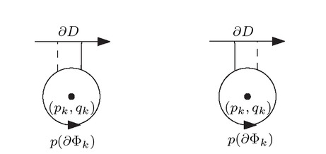
When b ≠ 0, the graph Γ_l, for l = 1, . . . , |b|, is depicted in Figure 8 (respectively Figure 9) for a fibre of type (1, 1) (respectively (1, −1)), just labelled by + (respectively −) inside the disk. If we take for δδ^′_l^′ the shifts induced by that of δ_l, then we can choose as region R_l the gray one, containing in its boundary all vertices of Γ_l belonging to ∂Φ_lexcept one (the thick points in the first two pictures). On the contrary, if one of the two shifts is changed as in the third draw of Figures 8 and 9, then R_l can be chosen containing in its boundary all the vertices of Γ_l belonging to ∂Φ_l^′.

Figure 8

The graph Γ_l, with b > 0, embedded in T_l = ∂Φ_lwith different choices of the shifts for δl′ and δl′′.

Figure 9

The graph Γ_l, with b < 0 embedded in Tl=∂Φl′ with different choices of the shifts for δl′ and δl′′.

We remark that changing the shift of a component of A changes the intersection between the corresponding element of W^′ and ∂𝒮 (which is a non-trivial theta graph) by a flip move (see Figure 1). We denote with P^′ the skeleton obtained by removing the regions R₀ and R_l from P^′, for l = 1, . . . , |b|.

In order to construct a skeleton for Φ_k for k = 1, . . . , r, consider the skeleton P_F depicted in Figure 10: it is a skeleton for T² × [0, 1] with one true vertex and such that θ₀ = P_F ∩ (T² × {0}) (the graph in the upper face) and θ₁ = P_F ∩ (T² × {1}) (the graph in the bottom face) are two theta graphs differing for a flip move. Denote with Θ_pk^/_qk the subset of Θ(T²), consisting of the theta graphs containing the slope corresponding to p_k/q_k ∈ ℚ∪{∞}. Let θ_pk^/_qk be the theta graph in Θ_pk^/_qk that is closest to θ⁺. The skeleton X_k for Φ_k is obtained by assembling several skeletons of type P_F connecting the theta graph P^′ ∩ Φ_k to a theta graph which is one step closer to θ⁺ than θ_pj^/_qj , with respect to the distance on Θ(T²); see [5]. The number of the required flips is either S(p_j , q_j) −2 or S(p_j , q_j)− 1 depending on the shift chosen for the corresponding component of A used in the construction of the skeleton P^′.We call the shift regular in the first case and singular in the second one (see Figure 11).

Figure 10

A skeleton for T² × [0, 1] connecting two theta graphs differing by a flip move.

Figure 11

Regular shift (on the left) and singular shift (on the right).

The skeleton P_S of S is obtained by assembling P^″ with X_k, via the identity, for k = 1, . . . , r.

4.2 Proof of Theorem 1

Here we prove our first result. To begin with we need to discuss how to fix the choices in the construction of the skeleton P_S previously described, when the Seifert fibre space S = (g, d, (p₁, q₁), . . . , (p_r , q_r), b) is a piece of a graph manifold having all gluing matrices different from ±H. According to the notation introduced at the beginning of Section 3, we have d = d⁺ + d⁻ since E^′ = ∅.

Remark 2

Let θ₊ and θ₋ be the theta graphs corresponding, respectively, to Δ₊ and Δ₋ in the Farey triangulation. The intersection of each boundary component of S with the skeleton P_S is either θ₊ or θ₋, depending whether the shift of the corresponding component δ of A has been chosen as depicted in the left or right part of Figure 12, respectively.

Figure 12

The two possible choices for the shift corresponding to components of ∂𝒮.

We always choose these shifts such that exactly d⁺ (respectively d⁻) components have θ₋ (respectively θ₊) as intersection with P_S. Suppose that m ≤ b ≤ M, where m = −r − h − d⁻ + 1 and M = h + d⁺ − 1. If b ≤ −1

we can choose p0(Φ1′),…,p0(Φ|b|′) as |b| disks between those marked with − in Figure 13. In this way: (i) we can remove a region from T₀ containing 6 vertices of Γ₀, (ii) we can remove from T_l a region R_l containing in its boundary all the vertices of the graph Γ_l (as in the third drawing of Figure 9), for each l = 1, . . . , |b|, and (iii) we can take all regular shifts in the skeletons X_k corresponding to the exceptional fibres, for k = 1, . . . , r. If b = 0 we do not have to remove any regular neighbourhood Φregular fibres but still (i) and (iii) hold. An analogous situation happens if b ≥ 1, but in this case in order to satisfy (i), (ii) and (iii) the fibres of type (1, 1) correspond to some of the disks marked with + in Figure 14. As a result, when m ≤ b ≤ M the polyhedron P_S has      3      ( d + r + 2 h − 2 ) + ∑ k = 1 r S p k / q k − 2 true vertices.

Figure 13

An optimal choice for the shifts corresponding to (1, −1)-fibres, when b = m ≤ 0.

Figure 14

An optimal choice for the shifts corresponding to (1, 1)-fibres, when b = M ≥ 0.

If b < m ≤ 0 (respectively b > M ≥ 0) then (i) and (iii) hold and there are exactly m−b (respectively b−M) tori in which we remove a region R_l containing in its boundary all the vertices of Γ_l except one (see the first two pictures of Figure 8 and 9). Finally, if either b < m = 1 or b > M = −1 then (i) does not hold so we remove a region from T₀ containing 5 vertices of Γ₀. Moreover, there are exactly |b| tori in which we remove a region R_l containing all the vertices of Γ_l except one and (iii) holds. Summing up, if b < m (respectively b > M) then the number of true vertices of P_S increases by m − b (respectively b − M) with respect to the case m ≤ b ≤ M.

As a consequence, P_S has 3 ( d + r + 2 h − 2 ) + ∑ k = 1 r S p k / q k − 2 + f m , M ( b ) true vertices.

Now let T = (V, E_T) be a spanning tree of G and consider the graphmanifold M_T (with boundary if T ≠ G). We will construct a skeleton P_MT for M_T by assembling skeletons of its Seifert pieces (constructed as above) with skeletons of thickened tori corresponding to edges of T. More precisely, for each e ∈ E T  let  T e ′ ⊂ ∂ S v e ′ and Te′′⊂∂SVe′′ be the boundaries attached by A_e. We construct a skeleton PAe for Te′′×I, and assemble P S v e ′ with P_Ae using the map Ae:Te′→Te′′=Te′′×{0} and PAe with PSve′′ with the identification Te′′×{1}=Te′′.

Given e ∈ E_T, let θ_e be the theta graph corresponding to A_eΔ₋. We construct the skeleton P_Ae by assembling flip blocks (see Figure 10) so that (i) PAe∩(Te′′×{0})=θe and (ii) PAe∩(Te′′×{1})=θ+. By Lemma 1 we have c_Ae = d(A_eΔ₋, Δ₊) = S(β_e/δ_e)− 1, so the number of flip blocks required to construct P_Ae , as well as the number of true vertices of P_Ae, is S(β_e/δ_e)− 1.

By Remark 2, we can construct the skeleton P_Sv having 3 d v + r v + 2 h v − 2 + ∑ k = 1 r v S p k / q k − 2 + f m v , M v b v true vertices. So P_MT has

∑ e ∈ E T S β e / δ e − 1 + ∑ v ∈ V 3 d v + r v + 2 h v − 2 + ∑ k = 1 r v S p k / q k − 2 + f m v , M v b v

true vertices.

For each e ∈ E \ E_T, the matrix A_e identifies two boundary components of M_T. Denote with M_T∪e the resulting manifold. Construct P_Ae such that  (i) PAe∩(Te′′×{0})=θe and (ii) PAe∩(Te′′×{1})=θ′,  where θ_’ is at distance one from θ₊ and is closer to θ_e than θ₊. The graphs θ_’ and θ₊ differ for a flip, since they correspond to adjacent triangles, and therefore, as shown in Figure 15, we have i(θ^′ , θ₊) = 2, where i( ⋅ , ⋅) denotes the geometric intersection (i.e., the minimum number of intersection points up to isotopy). Consider the polyhedron PMT∪PAe∪(Te′′×{1}): it is a skeleton for P_MT∪e. Since P_Ae consists of S(β_e/δ_e)−2 flip blocks and the graph θ₊ ∪ θ^′ has 6 vertices of degree greater than 2, the new polyhedron has 5+ S(β_e/δ_e)−1 true vertices more than P_MT. By repeating this construction for any e ∈ E \ E_T and observing that |E \ E_T| = |E| − |V| +1we get the statement.

Figure 15

The two intersections of two theta graphs differing by a flip move.

4.3 Proof of Theorem 2

As in the proof of Theorem 1, we start by constructing a skeleton P_MT for the graph manifold M_T (with boundary if T ≠ G). By Lemma 1 we have 0 = c_±H = d(±HΔ₋, Δ₋) = d(±HΔ₊, Δ₊), so whenever e∈ET′=E′, no flip block is required in P_Ae and we can assemble directly PSve′ with PSve′′. So, if Te′ and Te′′ denote, respectively, the boundary components of S_vand S_v" glued by A_e, we require that either (i) PSve′∩Te′=θ+and PSve′′∩Te′′=θ+or (ii) PSve′∩Te′=θ−and PSve′′∩Te′′=θ−. 

In order to take care of these two possibilities we use a function ψ : E^′ → {+, −}. If the shifts in the construction of PSve′ and PSve′′ are chosen so that (i) holds (respectively (ii) holds) set ψ(e) = − (respectively ψ(e) = +). Following the construction of Remark 2, with d+=dv++dv,ψ+and d−=dv−+dv,ψ−, we obtain a skeleton P_Sv with 3 d v + r v + 2 h v − 2 + ∑ k = 1 r v S p k / q k − 2 + f m v , M v b v true vertices. Thus the minimum number of true vertices of the skeleton P_MT of M_T is ∑ e ∈ E T ′ ′ S β e / δ e − 1 + ∑ v ∈ V 3 d v + r v + 2 h v − 2 + ∑ k = 1 r v S p k / q k − 2 + min_ψ∈Ψ{Σ_v∈V f_{mv ,Mv} (b_v)}.

Since all the matrices associated to the edges e ∉ E_T are different from ±H, starting from P_MT we can construct a spine for M as described in the proof of Theorem 1. This concludes the proof.

4.4 Proof of Theorem 3

Let T = (V, E_T)∈ 𝒪_G. Given ψ ∈ Ψ_T,we construct a skeleton P_MT for M_T as described in the proof of Theorem 2. If e ∈E′\ET′, then A_e = ±H and it glues together two toric boundary components Te′⊂∂Sve′ and Te′′⊂∂Sve′′ of MT.

Let θ e ′ , θ e ′ ′ = P S v e ′ ∩ T e ′ , P S v e ′ ′ ∩ T e ′ ′ . Since A_eΔ_± = Δ_± and i(θ₊, θ₊) = i(θ₋, θ₊) = i(θ₋, θ₋) = 2, we have to consider all possible cases of θe′,θe′′∈{ θ+,θ− }. If (θe′,θe′′)=(θ+,θ−) (respectively (θe′,θe′′)=(θ−,θ+) ) then we define ψ^′(e) = −+ (respectively ψ′(e)=+− ). If (θe′,θe′′)=(θ+,θ+)or (θe′,θe′′)=(θ−,θ−) we can use Remark 1 in order to obtain a better estimate for c(M). Indeed, if we replace the matrix A_e with A_eU^∓1 (respectively U^±1A_e), then b_v(respectively b_v" ) is replaced with b_v∓ 1 (respectively bve′′ ∓1 ), but anyway i(θ−′,θ−)=i(θ−′′,θ−)=i(θ+′,θ+)=i(θ+′′,θ+)=2, where θ−′,θ−′′,θ+′,θ+′′ are the theta graphs associated to the triangles A_eU⁻¹Δ₋, UA_eΔ₋, A_eUΔ₊, U⁻¹A_eΔ₊, respectively. Indeed, A_eU⁻¹Δ₋, UA_eΔ₋ are adjacent to Δ₋ and A_eUΔ₊, U⁻¹A_eΔ₊ are adjacent to Δ₊. More precisely, if we take (θe′,θe′′)=(θ−,θ−) and replace A_e with A_eU⁻¹ (respectively UA_e) we set ψ^′(e) = ++(respectively ψ^′(e) = +), while if we take (θe′,θe′′)=(θ+,θ+) and replace A_e with A_eU (respectively U⁻¹A_e) we set ψ^′(e) = −− (respectively ψ^′(e) = −). As a result, the skeleton P_MT determined by ψ∈ΨT and ψ′∈ΨT′ has

true vertices.

A spine for M is given by the union of P_MT with: (i) the skeleton PAe∪Te′′×{1} described in the proof of Theorem 1 and having 5 + (S(β_e/δ_e)− 1) true vertices for each e∈E″\ET′′, and (ii) the torus Te′′, containing 6 true vertices for each e∈E′\ET′. Since | E′\ET′ |+| E″\ET′′ |=| E\ET |=|E|−|V|+1 and | E′\ET′ |=Φ(G) we get the statement.

References

[1] F. Bonahon, Low-dimensional geometry, volume 49 of Student Mathematical Library. Amer. Math. Soc. 2009. MR2522946 Zbl 1176.5700110.1090/stml/049Search in Google Scholar
[2] A. Cattabriga, S. Matveev, M. Mulazzani, T. Nasybullov, On the complexity of non-orientable Seifert fibre spaces. Indiana Univ. Math. J. 69 (2020), 421–451. MR4084177 Zbl 1445.5700910.1512/iumj.2020.69.7848Search in Google Scholar
[3] A. T. Fomenko, S. V. Matveev, Algorithmic and computer methods for three-manifolds, volume 425 of Mathematics and its Applications. Kluwer 1997. MR1486574 Zbl 0885.5700910.1007/978-94-017-0699-5Search in Google Scholar
[4] E. Fominykh, M. Ovchinnikov, On the complexity of graph manifolds. Sib. Èlektron. Mat. Izv. 2 (2005), 190–191. MR2177992 Zbl 1150.57309Search in Google Scholar
[5] E. Fominykh, B. Wiest, Upper bounds for the complexity of torus knot complements. J. Knot Theory Ramifications 22 (2013), 1350053, 19 pages. MR3125892 Zbl 1290.5700310.1142/S0218216513500533Search in Google Scholar
[6] E. A. Fominykh, Upper complexity bounds for an infinite series of graph manifolds. Sib. Èlektron. Mat. Izv. 5 (2008), 215–228. MR2586633 Zbl 1299.57008Search in Google Scholar
[7] W. Jaco, H. Rubinstein, S. Tillmann, Minimal triangulations for an infinite family of lens spaces. J. Topol. 2 (2009), 157–180. MR2499441 Zbl 1227.5702610.1112/jtopol/jtp004Search in Google Scholar
[8] W. Jaco, J. H. Rubinstein, S. Tillmann, Coverings and minimal triangulations of 3-manifolds. Algebr. Geom. Topol. 11 (2011), 1257–1265. MR2801418 Zbl 1229.5701010.2140/agt.2011.11.1257Search in Google Scholar
[9] B. Martelli, C. Petronio, A new decomposition theorem for 3-manifolds. Illinois J. Math. 46 (2002), 755–780. MR1951239 Zbl 1033.5701110.1215/ijm/1258130983Search in Google Scholar
[10] B. Martelli, C. Petronio, Complexity of geometric three-manifolds. Geom. Dedicata 108 (2004), 15–69. MR2112664 Zbl 1068.5701110.1007/s10711-004-3181-xSearch in Google Scholar
[11] S. Matveev, Algorithmic topology and classification of 3-manifolds, volume 9 of Algorithms and Computation in Mathematics. Springer 2003. MR1997069 Zbl 1048.5700110.1007/978-3-662-05102-3Search in Google Scholar
[12] S. V. Matveev, The complexity of three-dimensional manifolds and their enumeration in the order of increasing complexity. (Russian) Dokl. Akad. Nauk SSSR 301 (1988), 280–283. English translation: Soviet Math. Dokl. 38 (1989), no. 1, 75–78. MR967821 Zbl 0674.57012Search in Google Scholar
[13] S. V. Matveev, Complexity theory of three-dimensional manifolds. Acta Appl. Math. 19 (1990), 101–130. MR1074221 Zbl 0724.5701210.1007/BF00049576Search in Google Scholar
[14] A. Y. Vesnin, S. V. Matveev, E. A. Fominykh, New aspects of the complexity theory of three-dimensional manifolds. (Russian) Uspekhi Mat. Nauk 73 (2018), no. 4(442), 53–102. English translation: Russian Math. Surveys 73 (2018), no. 4, 615–660. MR3833508 Zbl 0705782310.1070/RM9829Search in Google Scholar
[15] F. Waldhausen, Eine Klasse von 3-dimensionalen Mannigfaltigkeiten I. Invent. Math. 3 (1967), 308–333. MR235576 Zbl 0168.4450310.1007/BF01402956Search in Google Scholar
[16] F. Waldhausen, Eine Klasse von 3-dimensionalen Mannigfaltigkeiten II. Invent. Math. 4 (1967), 87–117. MR235576 Zbl 0168.4450310.1007/BF01425244Search in Google Scholar
© 2022 Alessia Cattabriga and Michele Mulazzani, published by De Gruyter
This work is licensed under the Creative Commons Attribution 4.0 International License.
Articles in the same Issue
- Frontmatter
- Ricci almost solitons with associated projective vector field
- Stein domains in ℂ2 with prescribed boundary
- Two examples of harmonic maps into spheres
- Numerical semigroups, polyhedra, and posets II: locating certain families of semigroups
- The moduli space of tropical curves with fixed Newton polygon
- On nilpotent automorphism groups of function fields
- Locally homogeneous non-gradient quasi-Einstein 3-manifolds
- Positive Ricci curvature on fiber bundles with compact structure group
- Rank one sheaves over quaternion algebras on Enriques surfaces