
Computerized quantification of pain drawings
-
Søren O’Neill

 ,
Tue Secher Jensen
,
Tue Secher Jensen

Abstract
Background and aims
Using a computer algorithm to quantify pain drawings could be useful, especially when large numbers of drawings need to be assessed. Whilst informal visual assessment of pain drawings can give clinicians a quick impression of the extent of pain and its location, formal quantification of pain drawings by computer for research purposes is not necessarily trivial. The current study compared seven different approaches to quantification in a large sample of clinical spinal pain drawings.
Methods
A large number (n = 55,720) of pain drawings were extracted from the SpineData database, a clinical registry of spinal pain patients in the Region of Southern Denmark. Drawings were analyzed both as pixel (raster) and vector based images, with different approaches based on the raw pain drawing, simple encircling polygons, convex-hull encircling polygons and discrete anatomical regions. Data were analyzed using principal component analysis, correlation and linear regression, as well as informal visual inspection of outlier pain drawings.
Results
Eighty-one percent of the variance could be explained by the first principal component, which we interpreted as the true score variance, i.e. the variance attributable to differences in pain area between individuals. The second principal component explained 10% of the variance and was loaded differentially by polygon-based methods and non-polygon-based methods. Correlations between the different approaches ranged from 0.66 to 1.00. Some approaches correlated so strongly as to be interchangeable, others tended to bias area estimates significantly. Visual inspection of outlier pain drawing indicated that when the different approaches to quantification yielded different results, characteristic patterns could be identified in the style and patterns of those pain drawings.
Conclusions
The different approaches reflected the same underlying construct (pain area), but could not be relied upon to produce the same area estimates and were affected by the interaction between drawing style and quantification approach. To some extend, the “correct” choice of quantification method is specific to and dictated by the style of each pain drawing. A differentiated approach is required in which the results of quantification and the drawing style are considered in combination. We provide suggestions for such differentiated approaches taking into account the nature of the drawing data (raster vs. vector) and the method of analysis (partly vs completely automated).
Implications
The chosen method of quantifying pain drawings in combination with the drawing style of the individual patient, can impact the resulting area estimate to a significant degree. These issues should be considered before undertaking computerized area estimation of pain drawings.
1 Introduction
Pain is a complex psycho-sensory experience, which cannot be meaningfully quantified in only a single measure. Instead, different tools are used to quantify different aspects of the pain experience. At face value, the pain drawing can be used to quantify pain extent/area and location.
However, determining the best way to quantify pain drawings is not straight-forward and a number of different methods have been described in the literature. These methods can be grouped as approaches based on (1) area approximation, and (2) number and location of anatomical regions – see Fig. 1 for illustrations. A third group of classification methods is based on specific scoring criteria, in which “points” are counted on the basis of “written comments”, “whole-body pain”, “non-organic pain”, etc. These criteria are purported to indicate psychological stress (see Ransford et al. [1]), but have been subject to some criticism [2], [3], [4] and they are not included in the current study because they do not quantify pain area as such.
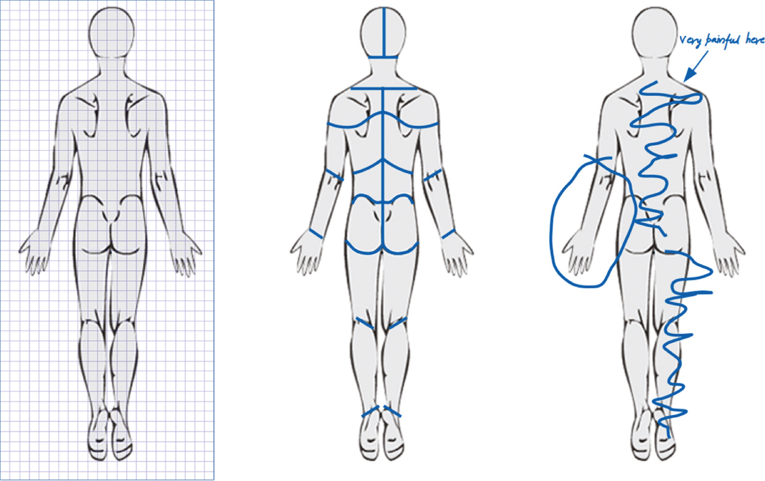
Stylized examples illustrating three distinct methods for quantifying pain drawings: Estimation of area (grid/pixels), counting of anatomical regions and scoring methods based on criteria such as “non-organic pain”, “whole body pain”, etc. (left-to-right).
With the first approach, approximation of the painful area is typically done by subdividing the pain drawing into a grid with squares of known size and simply counting the number of involved squares. In its most basic form, the empty pain drawing is printed onto common “squared graph paper” (see Ohlund et al. [5] for an example), whilst other methods have overlay grids specially adapted to the outline of the pain drawing (see Gatchel et al. [6]). Computerized analysis of digital drawings is typically performed in this manner, albeit with a much larger number of much smaller squares (pixels). Pain drawings can be stored on computers in two fundamentally different file formats: vector-based or pixel/raster-based. Pixel-based analysis was employed as early as 1991 by Mann et al. [7]. Vector-based analysis is less common as the data capture and analysis processes are more complex.
The second approach, using the number and location of anatomical regions, also consists of counting subdivisions of the pain drawing, but in this case, on the basis of anatomical divisions such as upper leg, lower leg, foot, etc. (see Margolis et al. [8] for an example). This method provides information about the anatomical regions involved in pain, rather than area as such. However, as each anatomical region can be weighted in accordance to their absolute area, it can be adapted to provide a measure of area as well. This does carry the potential risk of overestimating the area when only a minor portion of a large anatomical region is indicated as painful, as the entire area is included if any part is indicated as painful.
In a clinical setting, simple visual inspection of pain drawings probably suffices to get an overall impression of pain extent, location, etc. but for research there is a need to quantify pain drawings reliably. Moreover, when large amounts of pain drawing data have been collected in a digital format, it may be preferable to automate such quantification by use of a computer algorithm. However, this raises a number of potential issues:
Fig. 2 illustrates how automated analysis of pain drawings using the first approach could generate misleading results. The left panel of the figure illustrates a “raw pain drawing” and includes examples of pain indicated as a simple line-stroke (left shoulder), an encircled area (lower leg) and a hatched (criss-crossed) area (lumbar region). If the pain drawing in Fig. 2 is quantified by area approximation (pixel counting), the encircled and hatched areas would be significantly underestimated as only the pixels in the outline would be counted. Provided the pain drawing is stored in an appropriate vector-based format this problem can be overcome to some degree by simply “closing” the line-stroke – i.e. by connecting the start and end points of each stroke to form a simple polygon from which an area can be accurately calculated. As illustrated in the center panel of Fig. 2, this yields a good approximation for the encircled area but still underestimates the hatched pain area and, conversely, potentially overestimates the area from the simple line. For comparison, the right panel of the figure illustrates a more complex vector-based solution, which relies on calculating the “convex hull” polygon, i.e. the polygon with the least number of sides, which encapsulates the simple polygon. This method provides a good estimate for the hatched area but overestimates the encircled area of the lower leg and the line on the shoulder.
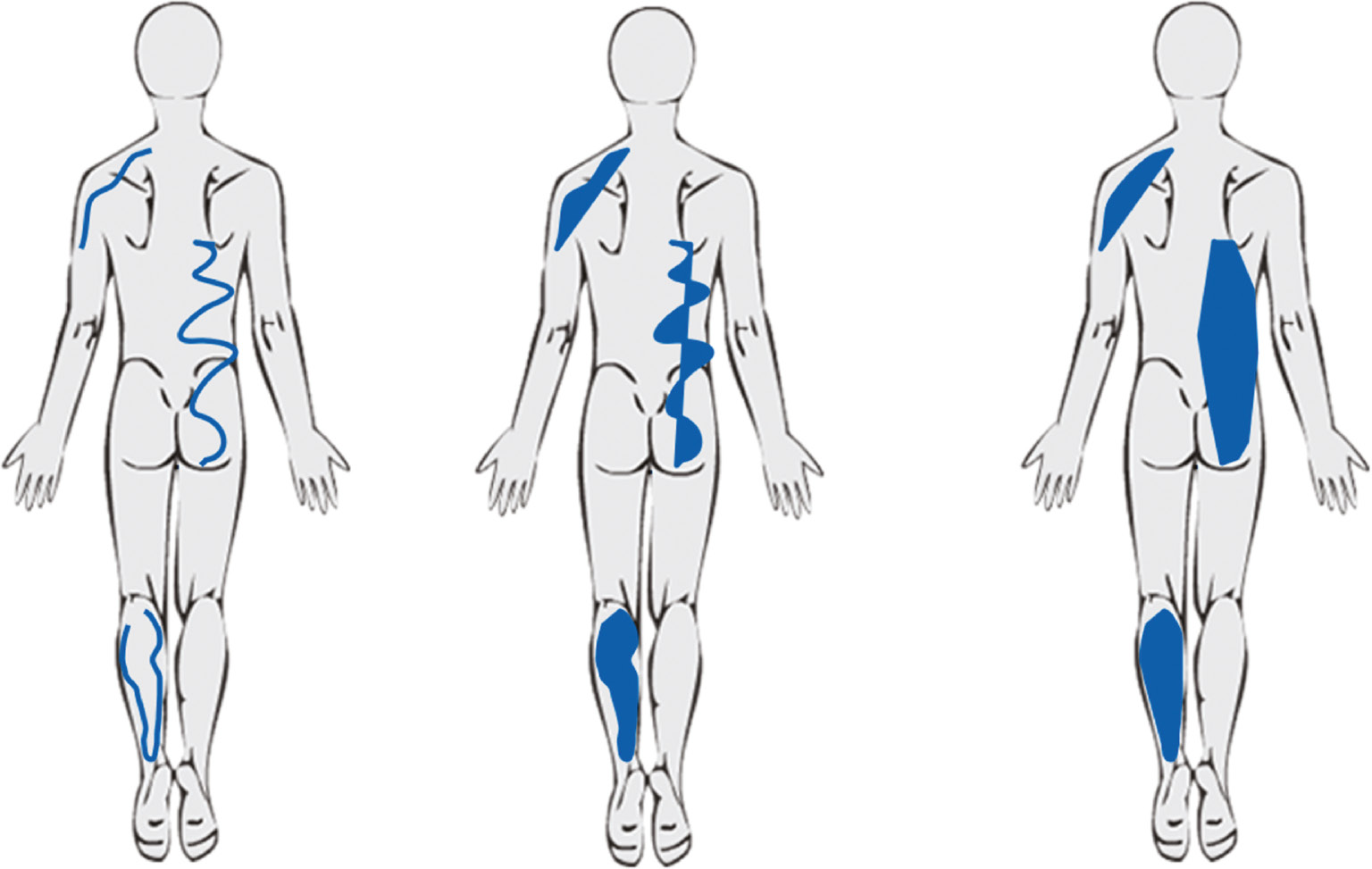
Constructed examples for illustrating potential problems when analyzing pain drawings. The left panel illustrates the raw pain drawing. The center panel illustrates the same drawing converted to simple, closed polygons and the right panel illustrates the convex hull polygons. Each method of area estimation has the potential for over- or underestimating the area.
The simple polygon and convex hull polygon examples (of the first approach) just described require data to be stored in a vector-based format. Such data may not always be available. Furthermore, such vector-based methods can potentially overestimate the area if the patient draws repeatedly in the same area resulting in overlapping polygons – unless such overlaps are corrected for. It is not self-evident which method provides the best summative estimate of painful areas and that may depend on the particulars of the individual pain drawing.
The counting of involved anatomical regions (the second approach) is a lot simpler to perform but also has limitations. For example, if the anatomical divisions illustrated in the center panel of Fig. 1 were used, the pain indicated in the left shoulder and right lumbar region of Fig. 2 would yield that same result of 3 involved regions, despite the obvious disparity in the two areas. It would be tempting to solve this issue by simply subdividing the pain drawing into a greater number of smaller anatomical regions but in essence this would just approach a pain area estimation method (the first approach) with the same potential issues as described above.
The automated quantification of pain drawings therefore needs to consider these issues and potential pitfalls in order to generate useful data.
Principal Components Analysis is a statistical method that can assist in understanding whether different measurement methods are measuring the same construct (a single dimension) or are measuring more than one dimension. Similarly, Spearmans correlations coefficients and the R2 from linear regression models provide information about the co-variance between different measures. In the present context, these three tools were potentially useful for understanding if these different ways of quantifying pain areas were measuring the same thing and the amount of similarity in their scores.
Therefore, the aim of the current study was to (a) use Principal Component Analysis, correlation coefficients and linear regression models to examine the co-variance between different computerized methods of quantifying pain drawing area, and (b) use visual inspection to identify and report where different methods of quantifying pain drawings yield different results.
2 Methods
2.1 Setting
Data were extracted from the SpineData Database [9] (Danish Data Protection Agency ref. no. 2000-53-0037) which is a clinical registry of patients with spinal pain syndromes. The database is used at the Spine Center of Southern Denmark, a large specialized hospital department in the region of Southern Denmark (total population 1.2 million). Patient referrals come from private practice clinicians (general medical practitioners, chiropractors and consultant medical specialists) as well as other hospital departments. Patients present almost exclusively with chronic spinal pain syndromes that have failed to respond sufficiently to conservative care in the primary care sector. All available relevant data was retrieved from the SpineData database for patients with an initial consultation between 23 February 2011 and 18 April 2018 with no restrictions on their clinical presentation.
2.2 Clinical data
Data were extracted from the database on patient sex, age, duration of pain and typical clinical pain intensity, as well as the region indicated by the patient as the main clinical pain area (neck, mid-back or low-back).
2.3 Acquisition of pain drawing data
The SpineData questionnaire includes a 450×500 pixel digital pain drawing template (see Fig. 3) on to which patients can draw with their finger when using a touch-screen, or with a computer mouse when using a regular computer. The computer interface was programmed with a fixed stroke-width of 5 pixels, i.e. a line drawn on the screen would have a standard width of 5 pixels, irrespective of whether the line was drawn using a computer mouse or a touch screen interface. Patients either completed the questionnaire on a digital tablet in the waiting room before their first consultation or online no earlier than 48 h prior to the appointment. No data was recorded about the method (mouse or touch screen) used.
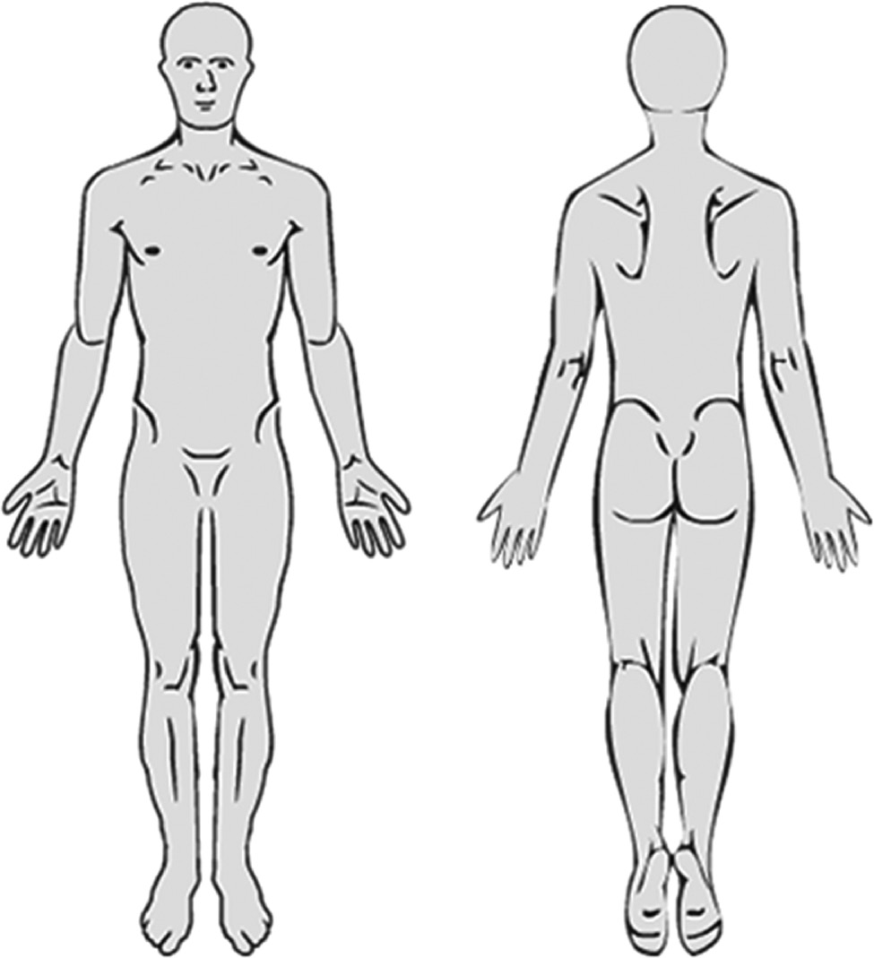
The pain drawing as presented to patients.
The pain drawing was stored as a scalable vector graphics (SVG) in extended markup language format (XML). The SVG code is a standard computer format for storing vector-based graphics, which in this case defines a Cartesian coordinate system (0–450×0–500) super-imposed on the template pain drawing (Fig. 3). The SVG code therefore represents a number of drawing “strokes” within that coordinate system, where each stroke defines a continuous path from start (“pen-down”) to finish (“pen-up”). This is quantified as a series of x,y-coordinates representing points along the stroke path. So, each pain drawing thus consisted of a variable number of strokes and each stroke was defined by a variable number of points in the coordinate system.
The drawing was also divided into 46 predefined rectangular anatomical regions roughly corresponding to: forehead, face, neck (right front), neck (left front), etc. – see Fig. 4. For each anatomical region, a simple unweighted dichotomous (true/false) variable was stored indicating whether or not the patients’ drawing involved that particular area. The anatomical subdivisions were not evident to the patients who only saw the plain pain drawing (Fig. 3).
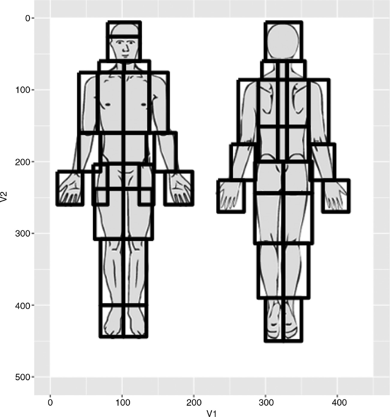
Anatomical subdivisions of the pain drawing.
2.4 Quantification of pain drawing data
Pain drawings were analyzed using two first approaches described in the introduction: pain area estimation and the counting of anatomical regions. Analysis was performed entirely by computer algorithms programmed in the statistical computing language R.
For each drawing, seven pain drawing variables were generated representing different quantification methods:
2.4.1 Pain area estimation variables
SVG stroke: Area was calculated based on the “raw data”, i.e. the actual SVG stroke definitions (with a stroke width of 5 pixels). So for each stroke the area was calculated as the combined length of the individual line segments ×5 and the total area for each drawing was calculated as a simple pixel sum of the stroke areas.
Pixelated stroke: The raw SVG definitions of each pain drawing were converted into a pixel/raster image of 450×500, in such a way that each pixel was either filled in or empty, i.e. without color gradients. The total area was calculated as the number of filled-in pixels.
SVG simple polygon: The area was calculated based on the SVG stroke definitions but each stroke was “closed” in such a way that a new, last “pen-up” coordinate was added as a copy of the starting “pen-down” coordinate, thus converting strokes into simple polygons. The geometric area was calculated for each polygon and the total area for each drawing was calculated as a simple sum of polygons. The additional area stemming from the 5 pixel stroke width was ignored.
Pixelated simple polygon: Each SVG stroke definition was converted to a closed and filled-in polygon and this SVG definition was converted to a pixel image of 450×500 pixels. The total area was calculated as the number of filled-in pixels.
SVG convex hull polygon: The area was calculated based on the convex hull method, in which the polygon with the smallest number of sides was calculated to encapsulate each stroke. The total area was calculated as the sum of the convex hull polygon areas.
Pixelated convex hull polygon: For each SVG stroke definition the convex hull polygon was calculated as a filled-in polygon and this SVG definition was converted to a pixel image of 450×500 pixels. The total area was calculated as the number of filled-in pixels.
In this manner, the area (in pixels) was estimated based on: the actual raw data strokes on the pain drawing (Methods 1 and 2) with a standard stroke width of 5 pixels; the simple polygons defined by those strokes (Methods 3 and 4); and the convex hull defined by the strokes (Methods 5 and 6). Methods 2, 4, and 6 (pixelated pain drawings) eliminated any additive effect of overlapping areas, whereas Methods 1, 3 and 5 (vectorized pain drawings) do not. The stroke-based methods (Methods 1 and 2) “added” an area corresponding to a standard stroke width of 5 pixels (as illustrated on the patient’s screen), whereas the polygon-based methods (Methods 3–6) calculated the absolute encapsulated geometrical area with no added stroke width. An R script of this analysis is provided as Supplementary Material.
2.4.2 Anatomical regions variable
An estimate of the area was calculated based on the anatomical regions involved (retrieved directly from the database), weighted using the absolute area of each anatomical region (see Appendix 1 and Fig. 4).
2.5 Statistical analysis
2.5.1 Descriptive and summary statistics
Descriptive and summary statistics are presented as both mean and standard deviation, as well as Tukeys five number summary (minimum, lower quartile, median, upper quartile and maximum) for non-parametric data. Formal testing for normality was performed with Shapiro-Wilk test, Kolmogorov-Smirnoff test and visual inspection of QQplots (not presented here). The Shapiro-Wilk test has been recommended over the Kolmogorov-Smirnoff test which has lower power. However, with large data sets, the Shapiro-Wilk test is disproportionately sensitive to even small deviations from the normal distribution and test was therefor performed on random samples (n=100 and n=1,000) of the full data set [10].
2.5.2 Principal component analysis
Principal component analysis results are summarized as standard deviation (sd), variance component and variable loading for the first two principal components. The variable loadings for the first and second principal component are presented on a standard principal component analysis plot. A scree-plot of Eigen values is presented for visual inspection.
2.5.3 Correlation and linear regression
Pair-wise comparisons of the seven pain drawing variables are quantified using correlation coefficients (Spearman’s ρ) and linear regression (R2 and residual SE).
2.6 Visual inspection
The 16 pain drawings with the highest degree of discrepancy between the most different quantification methods (as indicated by principal component analysis) are presented for informal visual inspection, thereby illustrating those pain drawings where the choice of quantification method made the biggest difference.
2.7 Ethics
Under Danish law, the secondary analysis of these de-identified registry data does not require ethics approval (The Act on Processing of Personal Data, December 2012, Section 5.2; Act on Research Ethics Review of Health Research Projects, October 2013, Section 14.2).
3 Results
3.1 Descriptive and summary statistics
Data from a total of 56,101 first-time visits were retrieved, but 381 contained coding errors in the SVG definitions (incomplete stroke elements), leaving 55,720 pain drawings for analysis. The analyzed cohort was comprised of 30,912 women of mean age 50.6 years [sd=15.4] and 24,808 men of mean age 51.1 years [sd=15.0].
The vast majority (76%) of patients reported low-back pain as the primary complaint, followed by neck pain (17%) and lastly, mid-back pain (7%). See Table 1 for summary statistics of clinical pain. For summary statistics of pain drawings see Table 2 and Fig. 5.
Summary clinical statistics.
| Location | n | Duration (days) | Typical pain (NRS) |
|---|---|---|---|
| Low back | 42,256 | 1,182 [2,242]{0; 120; 306; 1,096; 30,558} | 6.0 [2.4]{0; 5; 6; 8; 10} |
| Mid back | 4,114 | 1,119 [1,916]{0; 127; 365; 1,127; 17,532} | 6.3 [2.2]{0; 5; 7; 8; 10} |
| Neck | 9,350 | 936 [1,698]{0; 122; 292; 882; 30,542} | 6.0 [2.4]{0; 5; 6; 8; 10} |
-
Summary descriptive statistics. Duration and pain intensity is presented as mean [sd] {min, lower quartile, median, upper quartile, max}.
Summary pain drawing statistics.
| Location | Low back | Mid back | Neck |
|---|---|---|---|
| Strokes (n) | 8 [10]{1; 2; 5; 9; 201} | 8 [12]{1; 2; 5; 10; 226} | 10 [14]{1; 3; 6; 12; 385} |
| Stroke (SVG) | 2,177 [3,090]{5; 650; 1,400; 2,620; 103,015} | 2,345 [3,336]{5; 655; 1,417.5; 2,750; 54,405} | 2,539 [3,767]{5; 675; 1,530; 3,025; 90,020} |
| Polygon (SVG) | 1,730 [3,205]{0; 141; 617; 1,937; 68,162} | 2,189 [4,305]{0; 142; 712.5; 2,369; 70,891} | 1,943 [3,745]{0; 173; 773; 2,316; 169,762} |
| Convex hull (SVG) | 2,427 [3,920]{0; 266; 1,105; 2,957; 94,708} | 2,918 [5,006]{0; 259; 1,225.5; 3,531; 71,091} | 3,116 [5,282]{0; 312; 1,478; 3,892; 206,895} |
| Stroke (pixel) | 2,110 [2,158]{6; 709.5; 1,590; 2,790; 42,400} | 2,195 [2,330]{6; 705; 1,557; 2,769; 22,764} | 2,440 [2,689]{6; 753; 1,712; 3,223; 71,164} |
| Polygon (pixel) | 3,342 [4,020]{6; 851; 2,175; 4,323; 76,431} | 3,678 [4,894]{6; 826; 2,189; 4,707; 76,994} | 3,883 [4,671]{6; 924; 2,548; 5,104; 92,719} |
| Convex hull (pixel) | 3,840 [4,599]{6; 939; 2,481; 5,021.5; 100,959} | 4,199 [5,543]{6; 913; 2,458; 5,392; 77,327} | 4,687 [5,773]{6; 1,029; 2,981.5; 6,153; 98,768} |
| Anatomical regions (n) | 7 [5]{0; 4; 6; 9; 44} | 8 [6]{0; 4; 7; 10; 44} | 9 [6]{0; 5; 8; 11; 44} |
| Anatomical regions (pixel) | 12,995 [9,046]{0; 6,950; 10,827; 16,890; 78,778} | 12,990 [10,200]{0; 6,180; 10,500; 16,695; 78,553} | 14,229 [10,755]{0; 7,055; 11,376; 18,433; 78,018} |
-
Summary statistics of pain drawings. Columns list mean [sd] {min, lower quartile, median, upper quartile, max}.
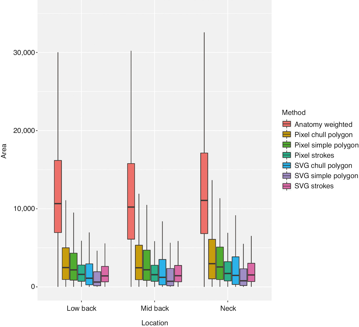
Box plot (non-parametric summary statistics) of pain drawing areas, by quantification method and bodily region. Outlier values have been omitted from plot for clarity.
As illustrated in Fig. 5, the pain drawing data distribution appears skewed by a predictable flooring effect. Formal testing (Shapiro-Wilk and Kolmogorov-Smirnoff) rejected the null-hypotheses that the seven variables were normally distributed (all p<0.0001).
3.2 Principal component analysis
Results of the principal component analysis (scaled) are presented in Tables 3 and 4 and Fig. 6. Eighty one percent of the variance could be explained by the first principal component (Table 3) and the seven variables had roughly equal loading on that component (0.32–0.41, see Table 4). The second principal component explained only 10% of the variance but with considerable differences in both magnitude and direction of loadings. A scree plot of Eigen values (Fig. 7) also illustrates that the data can be meaningfully described by a single underlying component.
Summary principal component analysis statistics.
| PC1 | PC2 | |
|---|---|---|
| Standard deviation | 2.4 | 0.85 |
| Proportion of variance | 0.81 | 0.1 |
| Cumulative proportion | 0.81 | 0.91 |
-
Summary of Principal Component Analysis.
Principal component analysis loadings.
| Variable | PC1 | PC2 |
|---|---|---|
| SVG stroke | 0.32 | 0.56 |
| SVG polygon | 0.36 | −0.51 |
| SVG convex hull | 0.40 | −0.30 |
| Pixel stroke | 0.40 | 0.34 |
| Pixel polygon | 0.41 | −0.20 |
| Pixel convex hull | 0.41 | −0.15 |
| Anatomical regions weighted | 0.34 | 0.40 |
-
Summary of Principal Component Analysis.
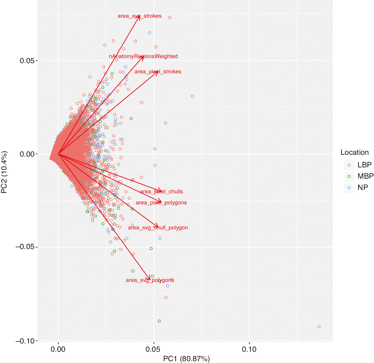
Bi-plot of principal component analysis components 1 and 2.
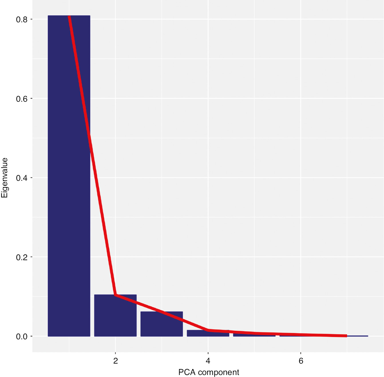
Scree plot of principal component analysis Eigen values demonstrating that the pain drawing variables can be meaningfully encapsulated in a single underlying principal component.
Based on the differential loading on the second principal component, two further analyses were performed as indicated by that differential loading:
Analysis of the four polygon-based variables in isolation indicated that the first principal component of that group explained 94% of the variance with equal loading by all four variables. The second component (only 4% variance) was differentially loaded by SVG based methods versus pixel-based methods.
Analysis of the other three variables (stroke SVG, stroke pixel and anatomical region) in isolation also indicated a first principal component with equal loading by all four variables, which explained 84% of the variance. The second component (14% variance) was differentially loaded by stroke-based methods versus the method based on anatomical regions.
3.3 Correlations and linear regression
Pair-wise correlation coefficients (Spearmans) and linear regression (R2 and residual standard error) are presented in Table 5.
Correlations and regression.
| svgStroke | svgPoly | svgChull | pixStroke | pixPoly | pixChull | wAnatomy | |
|---|---|---|---|---|---|---|---|
| svgStroke | 0.80 | 0.87 | 0.96 | 0.89 | 0.89 | 0.75 | |
| svgPoly | 0.25 [2,794] | 0.95 | 0.85 | 0.93 | 0.91 | 0.66 | |
| svgChull | 0.43 [2,449] | 0.85 [1,333] | 0.91 | 0.96 | 0.97 | 0.69 | |
| pixStroke | 0.73 [1,676] | 0.47 [2,479] | 0.66 [2,501] | 0.96 | 0.96 | 0.82 | |
| pixPoly | 0.40 [2,507] | 0.81 [1,475] | 0.88 [1,472] | 0.76 [1,116] | 1.00 | 0.79 | |
| pixChull | 0.42 [2,465] | 0.74 [1,725] | 0.90 [1,329] | 0.78 [1,060] | 0.97 [724] | 0.79 | |
| wAnatomy | 0.36 [2,595] | 0.28 [2,877] | 0.38 [3,373] | 0.68 [1,287] | 0.57 [2,769] | 0.57 [3,198] |
-
Table of correlation and linear regression. Spearmans correlation coefficients are presented in the upper-right part of the table (all significant at p<0.0001). The R2 [residual standard deviation] of a linear regression are presented in the lower-left half of the table.
3.4 Visual inspection of outliers
Based on the findings of the principal component analysis described above, the sum of the area quantified by the four polygon-based methods was calculated. Similarly, the sum area of the four non-polygon based methods was calculated and the sixteen drawings with the greatest difference in either direction were identified.
In a similar manner, we identified those drawings with the greatest degree of discrepancy in area between the two stroke-based methods and the anatomical region-based method.
The choice of pain drawings for visual inspection was guided by the results of principal component analysis and is presented in Figs. 8–11.

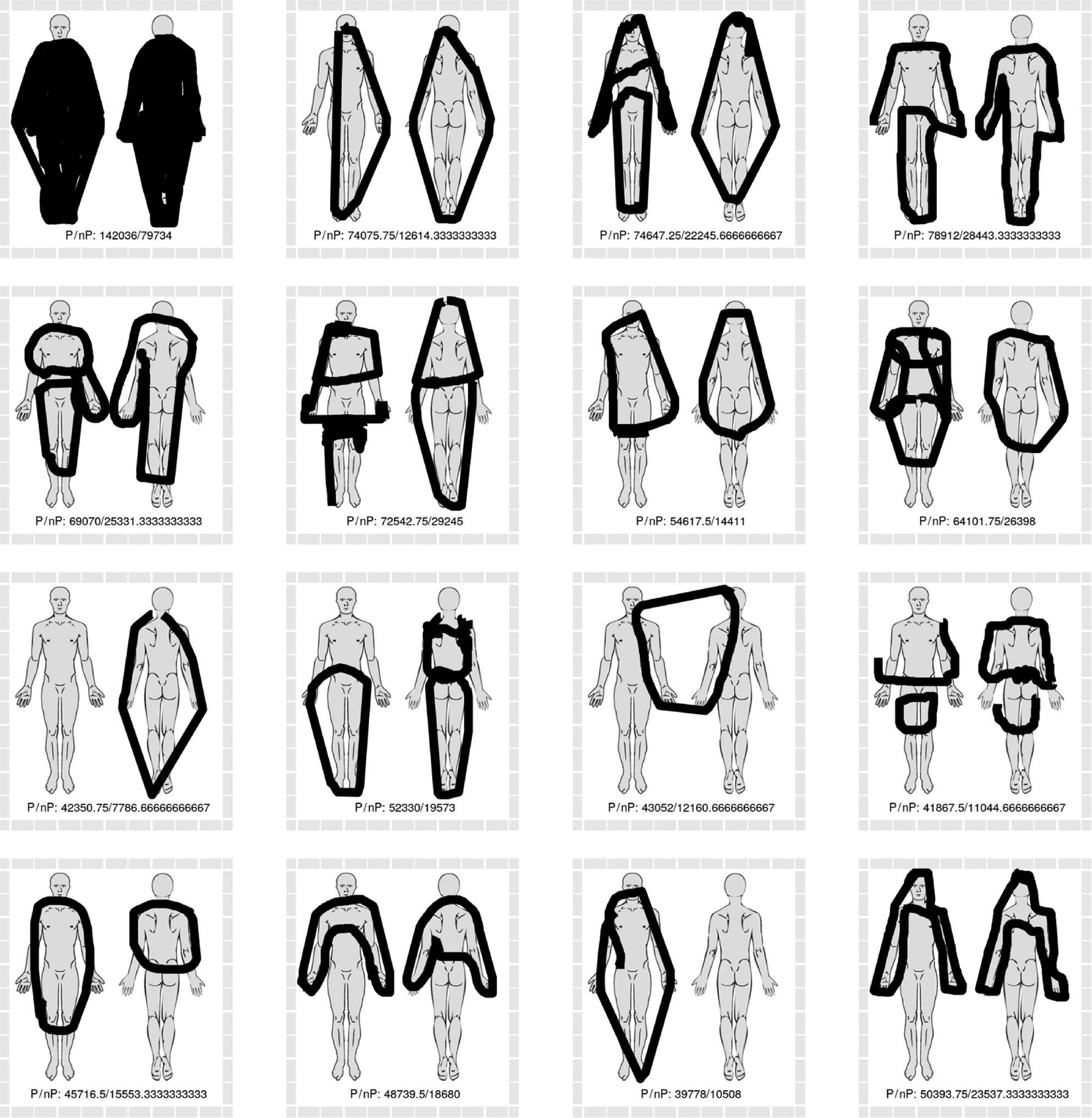
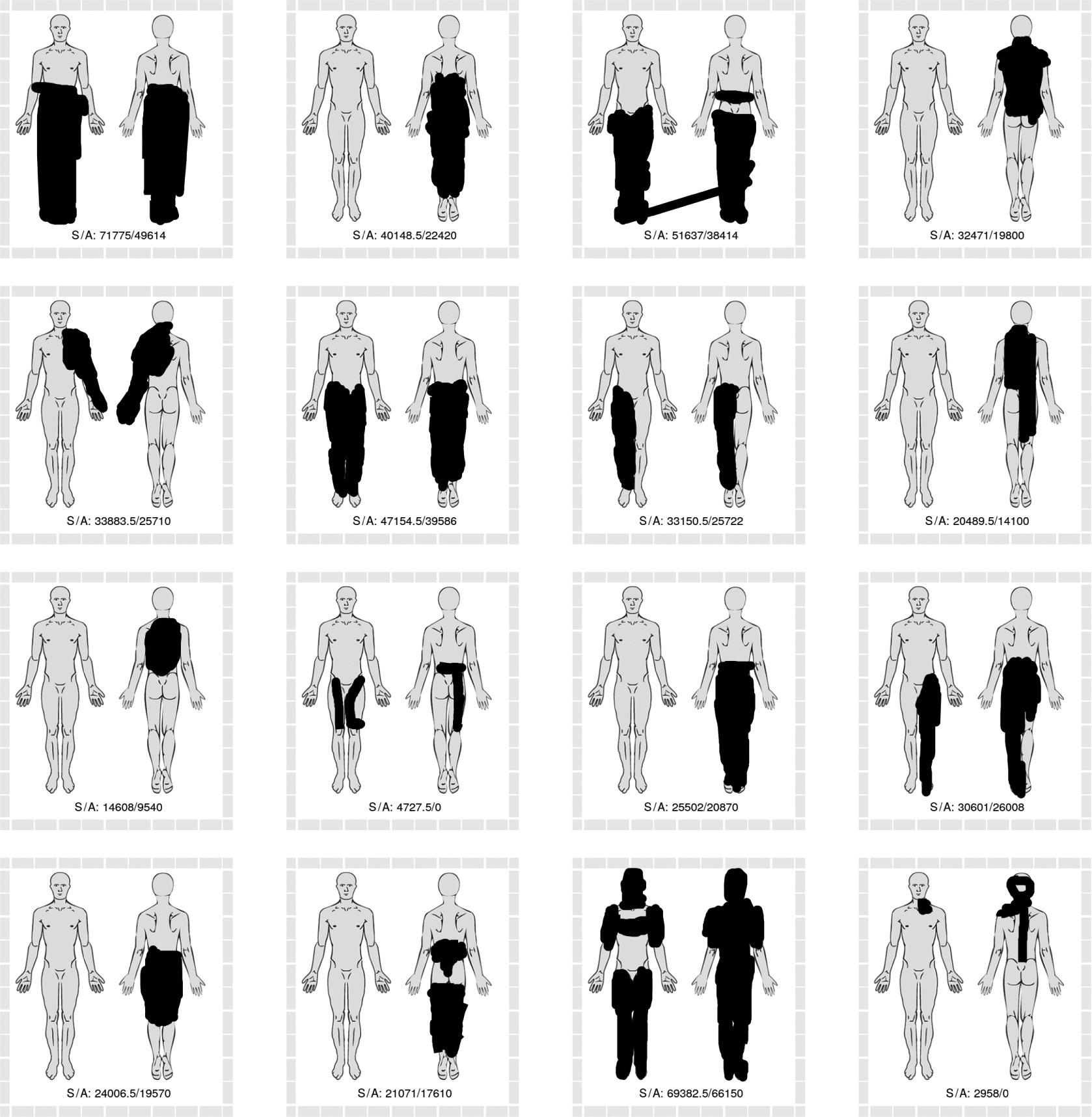
The sixteen pain drawings with the greatest discrepancy between polygon-based methods of area estimation (smaller area estimates) and non-polygon-based methods (greater area estimates). Numbers in drawing represent the area sum of the four polygon-based methods (P) and non-polygon-based methods (nP).
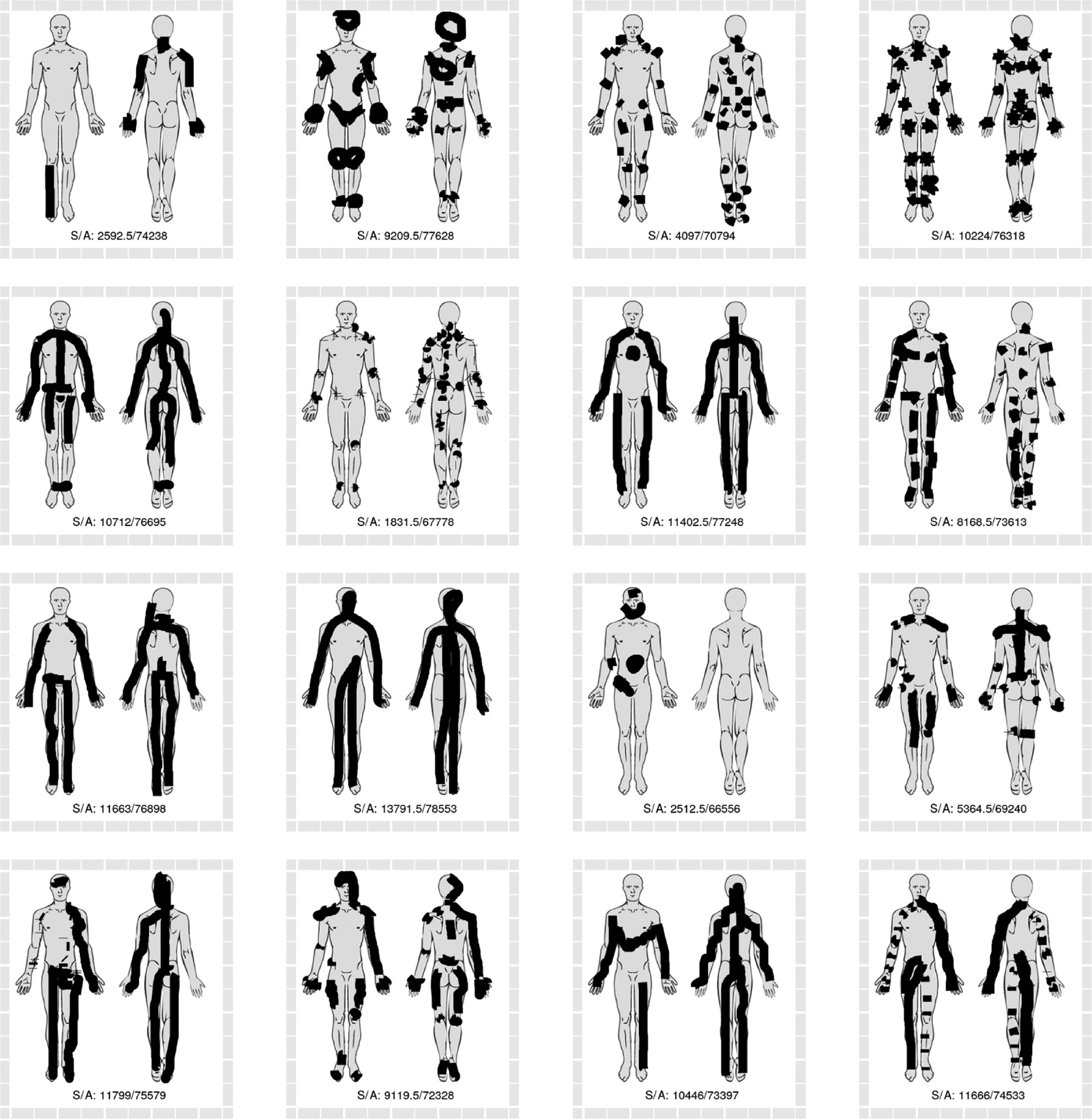
The sixteen pain drawings with the greatest discrepancy between polygon-based methods of area estimation (greater area estimates) and non-polygon-based methods (smaller area estimates). Numbers in drawing represent the area sum of the four polygon-based methods (P) and non-polygon-based methods (nP).
The sixteen pain drawings with the greatest discrepancy between methods based on raw SVG strokes (greater area estimates) and methods based on anatomical regions (lesser area estimates). Numbers in drawing represent the area sum of the two strokes-based methods (S) and anatomy-based methods (A). Two 0 values represent technical issues in data collection.
The sixteen pain drawings with the greatest discrepancy between methods based on raw SVG strokes (lesser area estimates) and methods based on anatomical regions (greater area estimates). Numbers in drawing represent the area sum of the two strokes based methods (S) and anatomy-based methods (A).
Visual inspection of pain drawings with high degrees of discrepancy between polygon-based and non-polygon-based methods revealed some obvious differences in drawing characteristics. Some patients indicated their pain to be in multiple sites, by use of many small drawing strokes (see Fig. 8). This style of drawing yielded relatively large area estimates with the non-polygon-based methods, due to the standard 5-pixel width of each stroke and relatively small circumscribed polygons. Conversely, the pain drawings with relatively large polygon-based area estimations (see Fig. 9) are characterized by a few strokes which circumscribe relatively large areas, in some instances extending beyond the body outline.
Comparing drawings with large discrepancy between stroke area (pixel or SVG) and weighted anatomical region estimates suggest that relatively large stroke area estimates are seen with many overlapping strokes within a relatively small anatomical area (see Fig. 10). Conversely, the drawings in Fig. 11 are characterized by either a few long strokes or a large number of small strokes, which include several anatomical regions.
4 Discussion
4.1 Principal component analysis
The first principal component explained most of the variability in the data (81%), which means that the multi-dimensional co-variability in the data could be meaningfully reduced to variability in a single dimension, albeit with some loss of information.
The results of a principal component analysis requires a contextual interpretation based on an understanding of the underlying data [11]: As all included variables had very similar loadings on the first principal component in the three principal component analyses, we interpret those components to represent the true score variance, i.e. actual variation in pain area between individuals. In other words, the principal component analysis indicates that all the employed methods quantify the same underlying construct: pain area. As mentioned, this accounted for most, but not all of the variation in our data.
The second principal component was loaded differentially by the seven variables, with those relying on polygon-based methods (simple polygon or convex hull, svg or pixel based) loading in the opposite direction of those based on the raw drawing strokes or anatomical regions (the direction is arbitrary and interchangeable in principal component analysis). This suggests that a distinction between those groups of methods may be important, although it still only accounts for a small degree of the variation (10%).
4.2 Correlation and linear modelling
Although the different methods of quantifying pain drawings generally had high coefficients of correlation (see Table 5), the goodness-of-fit and residual standard error of linear modelling suggest that different methods cannot be relied upon to generate the same measure of pain area.
The area estimates obtained through (weighted) counting of anatomical areas seem to have particularly low correlation and linear fit with the other methods. Table 2 and Fig. 5 indicate that this method systematically overestimates the pain area, which undoubtedly is because the entire anatomical region is counted even when only a smaller portion is actually indicated as painful.
As there is no gold standard for quantifying pain drawings, it is not obvious which method(s) most accurately quantifies the actual bodily extent of pain and, as described in the introduction, technical issues relating to the style of pain drawing may make one method more appropriate in some circumstances and less so in others.
4.3 Convex hull polygon method
The more complex method of using the convex hull polygon approach was included in the study to allow for examination of the effect of hatched areas. As discussed in the introduction, such pain drawings would likely result in significant discrepancy between that method and the simple polygon method. However, post-hoc visual analysis (not presented here) of the 16 drawings with the greatest discrepancy between simple polygon and convex hull polygon assessment did not reveal any such hatched pain drawings. We suspect the digital pain drawing interface does not encourage the participant to use hatching. Of course, this may be different with paper-based pain drawings.
4.4 Visual inspection of discrepant pain drawings
Visual inspection of pain drawings with greater degrees of discrepancy in area estimates, demonstrates discernible and characteristic patterns. The implication of this observation is, that the approach or method of area estimation cannot be made blindly, but must be guided in some way to allow for the _style_ of the individual pain drawing.
If the drawing style is not taken into consideration, an over- or underestimation of area in the region of 300% may be the result in extreme cases, such as those illustrated in Figs. 8–11.
5 Conclusions
This study demonstrated that computerized analysis of pain drawings is possible but the choice of method for quantifying the painful area can impact the results. There is no simple answer about which method provides the best area estimate, as considerable over/underestimation of area is seen with different combinations of methodology and drawing style.
However, convex hull polygon estimation of digital pain drawings can probably be omitted as the results are nearly identical to those of the simple polygon area estimation. Also, area estimation by summation of weighted anatomical regions seems likely to systematically overestimate the area in absolute numbers, albeit its results correlate well with other methods.
We suggest the following practical approach to computerized quantification of pain drawings:
If pain drawings are stored as pixel/raster data, each drawing must be manually examined to ensure that encircled areas are included in the area estimate.
If pain drawings are stored as vector data, firstly calculate both a simple polygon-based area estimate and an estimate based on the stroke area. Secondly, pragmatically use visual inspection to identify those drawings where the two methods are discrepant and choose the method least likely to over/underestimate the pain area. Alternatively, if analysis is only to be done by a computer algorithm:
select the strokes-based estimate if the polygon-based estimate is relatively large and number of strokes relatively small (corresponding to the situation in Fig. 9)
select the polygon-based method if the stroke-based estimate is relatively large and number of strokes relatively high (corresponding to the situation in Fig. 8).
Appendix 1: Weighted area of anatomical regions
| Note | Area |
|---|---|
| Front forehead | 900 |
| Front face | 1,530 |
| Front right neck | 560 |
| Front left neck | 560 |
| Front right arm | 2,184 |
| Front right chest | 3,024 |
| Front left chest | 3,024 |
| Front left arm | 2,184 |
| Front right forearm | 1,620 |
| Front right stomach | 1,376 |
| Front left stomach | 1,376 |
| Front left forearm | 1,620 |
| Front right hand | 1,610 |
| Front right groin | 770 |
| Front left groin | 770 |
| Front left hand | 1,748 |
| Front right thigh | 2,800 |
| Front left thigh | 2,800 |
| Front right leg | 2,944 |
| Front left leg | 2,944 |
| Front right foot | 1,408 |
| Front left foot | 1,408 |
| Back head | 2,700 |
| Back left neck | 572 |
| Back right neck | 650 |
| Back left arm | 2,520 |
| Back left thorasic | 1,755 |
| Back right thorasic | 1,950 |
| Back right arm | 2,520 |
| Back left forearm | 1,700 |
| Back left lower back | 1,323 |
| Back right lower back | 1,470 |
| Back right forearm | 1,700 |
| Back left hand | 1,584 |
| Back left buttock | 1,760 |
| Back right buttock | 1,760 |
| Back right hand | 1,584 |
| Back left thigh | 2,800 |
| Back right thigh | 2,800 |
| Back left calf | 2,660 |
| Back right calf | 2,660 |
| Back left foot | 1,500 |
| Back right foot | 1,500 |
| Mid back top | 338 |
| Mid back center | 845 |
| Mid back bottom | 637 |
-
Weighted area of pre-defined anatomical regions.
-
Authors’ statements
-
Research funding: The authors state that no external funding was involved in the present study.
-
Conflicts of interest: The authors state no conflicts of interest in the relation to the present study.
-
Informed consent: The authors state that that informed consent was obtained for all data in the present study.
-
Ethics approval: The authors state that the current study was conducted in accordance with the national ethics regulations and in accordance with the tenets of the Declaration of Helsinki. The regional ethics review board has approved the SpineData database.
References
[1] Ransford AO, Cairns D, Mooney V. The pain drawing as an aid to the psychologic evaluation of patients with low-back pain. Spine 1976;1:127–34.10.1097/00007632-197606000-00007Search in Google Scholar
[2] Von Baeyer CL, Bergstrom KJ, Brodwin MG, Brodwin SK. Invalid use of pain drawings in psychological screening of back pain patients. Pain 1983;16:103–7.10.1016/0304-3959(83)90089-1Search in Google Scholar PubMed
[3] Hildebrandt J, Franz CE, Choroba-Mehnen B, Temme M. The use of pain drawings in screening for psychological involvement in complaints of low-back pain. Spine 1988;13:681–5.10.1097/00007632-198813060-00016Search in Google Scholar
[4] Pfingsten M, Baller M, Liebeck H, Strube J, Hildebrandt J, Schops P. [Psychometric properties of the pain drawing and the Ransford technique in patients with chronic low back pain]. Schmerz 2003;17:332–40.10.1007/s00482-003-0223-0Search in Google Scholar PubMed
[5] Ohlund C, Eek C, Palmbald S, Areskoug B, Nachemson A. Quantified pain drawing in subacute low back pain. Validation in a nonselected outpatient industrial sample. Spine 1996;21:1021–30; discussion 1031.10.1097/00007632-199605010-00005Search in Google Scholar PubMed
[6] Gatchel RJ, Mayer TG, Capra P, Diamond P, Barnett J. Quantification of lumbar function. Part 6: the use of psychological measures in guiding physical functional restoration. Spine 1986;11:36–42.10.1097/00007632-198601000-00010Search in Google Scholar
[7] Mann III NH, Brown MD, Enger I. Statistical diagnosis of lumbar spine disorders using computerized patient pain drawings. Comput Biol Med 1991;21:383–97.10.1016/0010-4825(91)90040-GSearch in Google Scholar
[8] Margolis RB, Tait RC, Krause SJ. A rating system for use with patient pain drawings. Pain 1986;24:57–65.10.1016/0304-3959(86)90026-6Search in Google Scholar PubMed
[9] Kent P, Kongsted A, Jensen TS, Albert HB, Schiøttz-Christensen B, Manniche C. SpineData a Danish clinical registry of people with chronic back pain. Clin Epidemiol 2015;7: 369–80.10.2147/CLEP.S83830Search in Google Scholar PubMed PubMed Central
[10] Ghasemi A, Zahediasl S. Normality tests for statistical analysis: a guide for non-statisticians. Int J Endocrinol Metab 2012;10:486–9.10.5812/ijem.3505Search in Google Scholar PubMed PubMed Central
[11] Cadima J, Jolliffe IT. Loading and correlations in the interpretation of principle compenents. J Appl Stat 1995;22: 203–14.10.1080/757584614Search in Google Scholar
Supplementary Material
The online version of this article offers supplementary material (https://doi.org/10.1515/sjpain-2019-0082).
©2020 Scandinavian Association for the Study of Pain. Published by Walter de Gruyter GmbH, Berlin/Boston. All rights reserved.
Articles in the same Issue
- Frontmatter
- Editorial
- Change in Editorship: A Tribute to the Outgoing Editor-in-Chief
- Editorial comments
- Laboratory biomarkers of systemic inflammation – what can they tell us about chronic pain?
- Considering the interpersonal context of pain catastrophizing
- Systematic review
- Altered pain processing and sensitisation is evident in adults with patellofemoral pain: a systematic review including meta-analysis and meta-regression
- Topical reviews
- Pain revised – learning from anomalies
- Role of the immune system in neuropathic pain
- Clinical pain research
- Cryoneurolysis for cervicogenic headache – a double blinded randomized controlled study
- Interpersonal problems as a predictor of pain catastrophizing in patients with chronic pain
- Pain and small-fiber affection in hereditary neuropathy with liability to pressure palsies (HNPP)
- Predicting the outcome of persistent sciatica using conditioned pain modulation: 1-year results from a prospective cohort study
- Observational studies
- Revised chronic widespread pain criteria: development from and integration with fibromyalgia criteria
- The relationship between patient factors and the refusal of analgesics in adult Emergency Department patients with extremity injuries, a case-control study
- Chronic neuropathic pain after traumatic peripheral nerve injuries in the upper extremity: prevalence, demographic and surgical determinants, impact on health and on pain medication
- Tramadol prescribed use in general and chronic noncancer pain: a nationwide register-based cohort study of all patients above 16 years
- Changes in inflammatory plasma proteins from patients with chronic pain associated with treatment in an interdisciplinary multimodal rehabilitation program – an explorative multivariate pilot study
- Original experimental
- The pro-algesic effect of γ-aminobutyric acid (GABA) injection into the masseter muscle of healthy men and women
- The relationship between fear generalization and pain modulation: an investigation in healthy participants
- Experimental shoulder pain models do not validly replicate the clinical experience of shoulder pain
- Computerized quantification of pain drawings
- Head repositioning accuracy is influenced by experimental neck pain in those most accurate but not when adding a cognitive task
- Short communications
- Dispositional empathy is associated with experimental pain reduction during provision of social support by romantic partners
- Superior cervical sympathetic ganglion block under ultrasound guidance promotes recovery of abducens nerve palsy caused by microvascular ischemia